Transmission line

This article is about the radio-frequency transmission line. For the power transmission line, see electric power transmission.

In communications and electronic engineering, a transmission line is a specialized cable designed to carry alternating current of radio frequency, that is, currents with a frequency high enough that its wave nature must be taken into account. Transmission lines are used for purposes such as connecting radio transmitters and receivers with their antennas, distributing cable television signals, and computer network connections.

Explanation

Ordinary electrical cables suffice to carry low frequency AC, such as mains power, which reverses direction 100 to 120 times per second (cycling 50 to 60 times per second). However, they cannot be used to carry currents in the radio frequency range or higher, which reverse direction millions to billions of times per second, because the energy tends to radiate off the cable as radio waves, causing power losses. Radio frequency currents also tend to reflect from discontinuities in the cable such as connectors, and travel back down the cable toward the source. These reflections act as bottlenecks, preventing the power from reaching the destination. Transmission lines use specialized construction such as precise conductor dimensions and spacing, and impedance matching, to carry electromagnetic signals with minimal reflections and power losses. Types of transmission line include ladder line, coaxial cable, dielectric slabs, stripline, optical fiber, and waveguides. The higher the frequency, the shorter are the waves in a transmission medium. Transmission lines must be used when the frequency is high enough that the wavelength of the waves begins to approach the length of the cable used. To conduct energy at frequencies above the radio range, such as millimeter waves, infrared, and light, the waves become much smaller than the dimensions of the structures used to guide them, so transmission line techniques become inadequate and the methods of optics are used.

The theory of sound wave propagation is very similar mathematically to that of electromagnetic waves, so techniques from transmission line theory are also used to build structures to conduct acoustic waves; and these are also called transmission lines.

History

Mathematical analysis of the behaviour of electrical transmission lines grew out of the work of James Clerk Maxwell, Lord Kelvin and Oliver Heaviside. In 1855 Lord Kelvin formulated a diffusion model of the current in a submarine cable. The model correctly predicted the poor performance of the 1858 trans-Atlantic submarine telegraph cable. In 1885 Heaviside published the first papers that described his analysis of propagation in cables and the modern form of the telegrapher's equations.^[1]

Applicability

In many electric circuits, the length of the wires connecting the components can for the most part be ignored. That is, the voltage on the wire at a given time can be assumed to be the same at all points. However, when the voltage changes in a time interval comparable to the time it takes for the signal to travel down the wire, the length becomes important and the wire must be treated as a transmission line. Stated another way, the length of the wire is important when the signal includes frequency components with corresponding wavelengths comparable to or less than the length of the wire.

A common rule of thumb is that the cable or wire should be treated as a transmission line if the length is greater than 1/10 of the wavelength. At this length the phase delay and the interference of any reflections on the line become important and can lead to unpredictable behavior in systems which have not been carefully designed using transmission line theory.

The four terminal model

Variations on the schematic electronic symbol for a transmission line.

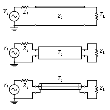
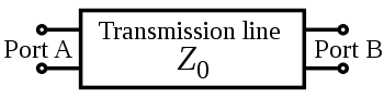
For the purposes of analysis, an electrical transmission line can be modelled as a two-port network (also called a quadrupole network), as follows:

In the simplest case, the network is assumed to be linear (i.e. the complex voltage across either port is proportional to the complex current flowing into it when there are no reflections), and the two ports are assumed to be interchangeable. If the transmission line is uniform along its length, then its behaviour is largely described by a single parameter called the characteristic impedance, symbol Z₀. This is the ratio of the complex voltage of a given wave to the complex current of the same wave at any point on the line. Typical values of Z₀ are 50 or 75 ohms for a coaxial cable, about 100 ohms for a twisted pair of wires, and about 300 ohms for a common type of untwisted pair used in radio transmission.

When sending power down a transmission line, it is usually desirable that as much power as possible will be absorbed by the load and as little as possible will be reflected back to the source. This can be ensured by making the load impedance equal to Z₀, in which case the transmission line is said to be matched.

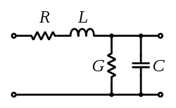
Some of the power that is fed into a transmission line is lost because of its resistance. This effect is called ohmic or resistive loss (see ohmic heating). At high frequencies, another effect called dielectric loss becomes significant, adding to the losses caused by resistance. Dielectric loss is caused when the insulating material inside the transmission line absorbs energy from the alternating electric field and converts it to heat (see dielectric heating). The Transmission Line is modeled with a Resistance(R) and Inductance(L) in Series with a Capacitance(C) and Conductance(G) in Parallel. The Resistance and Conductance contributes to the loss of the Transmission Line.

The total loss of power in a transmission line is often specified in decibels per metre (dB/m), and usually depends on the frequency of the signal. The manufacturer often supplies a chart showing the loss in dB/m at a range of frequencies. A loss of 3 dB corresponds approximately to a halving of the power.

High-frequency transmission lines can be defined as those designed to carry electromagnetic waves whose wavelengths are shorter than or comparable to the length of the line. Under these conditions, the approximations useful for calculations at lower frequencies are no longer accurate. This often occurs with radio, microwave and optical signals, metal mesh optical filters, and with the signals found in high-speed digital circuits.

Telegrapher's equations

Main article: Telegrapher's equations

See also: Reflections on copper lines

The Telegrapher's Equations (or just Telegraph Equations) are a pair of linear differential equations which describe the voltage and current on an electrical transmission line with distance and time. They were developed by Oliver Heaviside who created the transmission line model, and are based on Maxwell's Equations.

Schematic representation of the elementary component of a transmission line.

The transmission line model represents the transmission line as an infinite series of two-port elementary components, each representing an infinitesimally short segment of the transmission line:

• The distributed resistance R of the conductors is represented by a series resistor (expressed in ohms per unit length).
• The distributed inductance L (due to the magnetic field around the wires, self-inductance, etc.) is represented by a series inductor (henries per unit length).
• The capacitance C between the two conductors is represented by a shunt capacitor C (farads per unit length).
• The conductance G of the dielectric material separating the two conductors is represented by a shunt resistor between the signal wire and the return wire (siemens per unit length).

The model consists of an infinite series of the elements shown in the figure, and that the values of the components are specified per unit length so the picture of the component can be misleading. R, L, C, and G may also be functions of frequency. An alternative notation is to use R', L', C' and G' to emphasize that the values are derivatives with respect to length. These quantities can also be known as the primary line constants to distinguish from the secondary line constants derived from them, these being the propagation constant, attenuation constant and phase constant.

The line voltage V(x) and the current I(x) can be expressed in the frequency domain as

$\frac{\partial V(x)}{\partial x} = -(R + j \omega L)I(x)$

$\frac{\partial I(x)}{\partial x} = -(G + j \omega C)V(x).$

When the elements R and G are negligibly small the transmission line is considered as a lossless structure. In this hypothetical case, the model depends only on the L and C elements which greatly simplifies the analysis. For a lossless transmission line, the second order steady-state Telegrapher's equations are:

$\frac{\partial^2V(x)}{\partial x^2}+ \omega^2 LC\cdot V(x)=0$

$\frac{\partial^2I(x)}{\partial x^2} + \omega^2 LC\cdot I(x)=0.$

These are wave equations which have plane waves with equal propagation speed in the forward and reverse directions as solutions. The physical significance of this is that electromagnetic waves propagate down transmission lines and in general, there is a reflected component that interferes with the original signal. These equations are fundamental to transmission line theory.

If R and G are not neglected, the Telegrapher's equations become:

$\frac{\partial^2V(x)}{\partial x^2} = \gamma^2 V(x)$

$\frac{\partial^2I(x)}{\partial x^2} = \gamma^2 I(x)$

where

$\gamma = \sqrt{(R + j \omega L)(G + j \omega C)}$

and the characteristic impedance is:

$Z_0 = \sqrt{\frac{R + j \omega L}{G + j \omega C}}.$

The solutions for V(x) and I(x) are:

$V(x) = V^+ e^{-\gamma x} + V^- e^{\gamma x} \,$

$I(x) = \frac{1}{Z_0}(V^+ e^{-\gamma x} - V^- e^{\gamma x}). \,$

The constants $V^\pm$ and $I^\pm$ must be determined from boundary conditions. For a voltage pulse $V_{\mathrm{in}}(t) \,$, starting at x = 0 and moving in the positive x-direction, then the transmitted pulse $V_{\mathrm{out}}(x,t) \,$ at position x can be obtained by computing the Fourier Transform, $\tilde{V}(\omega)$, of $V_{\mathrm{in}}(t) \,$, attenuating each frequency component by $e^{\mathrm{-Re}(\gamma) x} \,$, advancing its phase by $\mathrm{-Im}(\gamma)x \,$, and taking the inverse Fourier Transform. The real and imaginary parts of γ can be computed as

$\mathrm{Re}(\gamma) = (a^2 + b^2)^{1/4} \cos(\mathrm{atan2}(b,a)/2) \,$

$\mathrm{Im}(\gamma) = (a^2 + b^2)^{1/4} \sin(\mathrm{atan2}(b,a)/2) \,$

where atan2 is the two-parameter arctangent, and

$a \equiv \omega^2 LC \left[ \left( \frac{R}{\omega L} \right) \left( \frac{G}{\omega C} \right) - 1 \right]$

$b \equiv \omega^2 LC \left( \frac{R}{\omega L} + \frac{G}{\omega C} \right).$

For small losses and high frequencies, to first order in R / ωL and G / ωC one obtains

$\mathrm{Re}(\gamma) \approx \frac{\sqrt{LC}}{2} \left( \frac{R}{L} + \frac{G}{C} \right) \,$

$\mathrm{Im}(\gamma) \approx \omega \sqrt{LC}. \,$

Noting that an advance in phase by − ωδ is equivalent to a time delay by δ, V_out(t) can be simply computed as

$V_{\mathrm{out}}(x,t) \approx V_{\mathrm{in}}(t - \sqrt{LC}x) e^{- \frac{\sqrt{LC}}{2} \left( \frac{R}{L} + \frac{G}{C} \right) x }. \,$

Input impedance of lossless transmission line

The characteristic impedance Z₀ of a transmission line is the ratio of the amplitude of a single voltage wave to its current wave. Since most transmission lines also have a reflected wave, the characteristic impedance is generally not the impedance that is measured on the line.

For a lossless transmission line, it can be shown that the impedance measured at a given position l from the load impedance Z_L is

$Z_\mathrm{in} (l)=Z_0 \frac{Z_L + jZ_0\tan(\beta l)}{Z_0 + jZ_L\tan(\beta l)}$

where $\beta=\frac{2\pi}{\lambda}$ is the wavenumber.

In calculating β, the wavelength is generally different inside the transmission line to what it would be in free-space and the velocity constant of the material the transmission line is made of needs to be taken into account when doing such a calculation.

Special cases

Half wave length

For the special case where βl = nπ where n is an integer (meaning that the length of the line is a multiple of half a wavelength), the expression reduces to the load impedance so that

$Z_\mathrm{in}=Z_L \,$

for all n. This includes the case when n = 0, meaning that the length of the transmission line is negligibly small compared to the wavelength. The physical significance of this is that the transmission line can be ignored (i.e. treated as a wire) in either case.

Quarter wave length

Main article: quarter wave impedance transformer

For the case where the length of the line is one quarter wavelength long, or an odd multiple of a quarter wavelength long, the input impedance becomes

$Z_\mathrm{in}=\frac{{Z_0}^2}{Z_L}. \,$

Matched load

Another special case is when the load impedance is equal to the characteristic impedance of the line (i.e. the line is matched), in which case the impedance reduces to the characteristic impedance of the line so that

$Z_\mathrm{in}=Z_L=Z_0 \,$

for all l and all λ.

Short

Main article: stub

For the case of a shorted load (i.e. Z_L = 0), the input impedance is purely imaginary and a periodic function of position and wavelength (frequency)

$Z_\mathrm{in} (l)=j Z_0 \tan(\beta l). \,$

Open

Main article: stub

For the case of an open load (i.e. $Z_L=\infty$), the input impedance is once again imaginary and periodic

$Z_\mathrm{in} (l)=-j Z_0 \cot(\beta l). \,$

Stepped transmission line

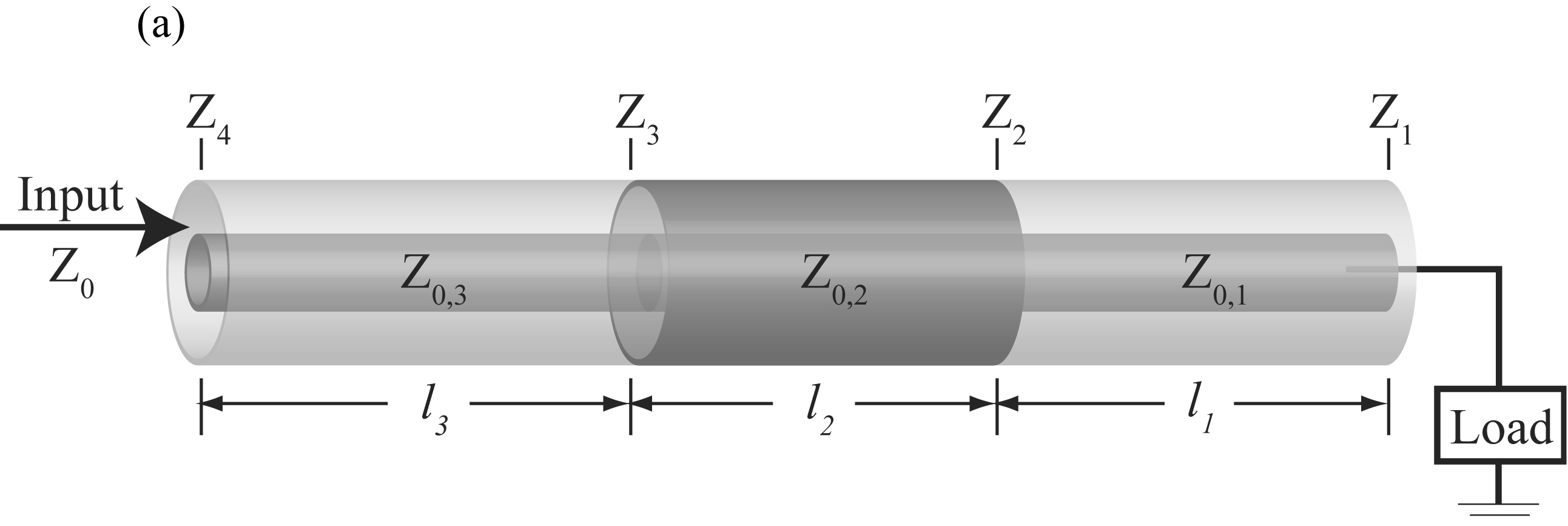
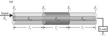A simple example of stepped transmission line consisting of three segments.

Stepped transmission line is used for broad range impedance matching. It can be considered as multiple transmission line segments connected in serial, with the characteristic impedance of each individual element to be, Z_0,i. And the input impedance can be obtained from the successive application of the chain relation

$Z_\mathrm{i+1}=Z_\mathrm{0,i} \frac{Z_i + jZ_\mathrm{0,i}\tan(\beta_i l_i)}{Z_\mathrm{0,i} + jZ_i\tan(\beta_i l_i)}$

where β_i is the wave number of the ith transmission line segment and l_i is the length of this segment, and Z_i is the front-end impedance that loads the ith segment.

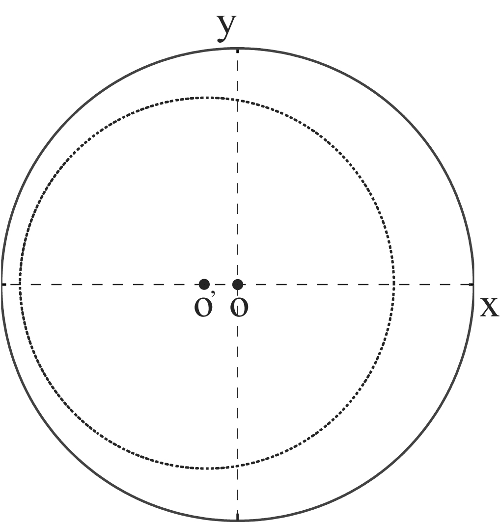
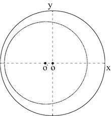The impedance transformation circle along a transmission line whose characteristic impedance Z_0,i is smaller than that of the input cable Z₀. And as a result, the impedance curve is off-centered towards the -x axis. Conversely, if Z_0,i > Z₀, the impedance curve should be off-centered towards the +x axis.

Because the characteristic impedance of each transmission line segment Z_0,i is often different from that of the input cable Z₀, the impedance transformation circle is off centered along the x axis of the Smith Chart whose impedance representation is usually normalized against Z₀.

Practical types

Coaxial cable

Main article: coaxial cable

Coaxial lines confine virtually all of the electromagnetic wave to the area inside the cable. Coaxial lines can therefore be bent and twisted (subject to limits) without negative effects, and they can be strapped to conductive supports without inducing unwanted currents in them. In radio-frequency applications up to a few gigahertz, the wave propagates in the transverse electric and magnetic mode (TEM) only, which means that the electric and magnetic fields are both perpendicular to the direction of propagation (the electric field is radial, and the magnetic field is circumferential). However, at frequencies for which the wavelength (in the dielectric) is significantly shorter than the circumference of the cable, transverse electric (TE) and transverse magnetic (TM) waveguide modes can also propagate. When more than one mode can exist, bends and other irregularities in the cable geometry can cause power to be transferred from one mode to another.

The most common use for coaxial cables is for television and other signals with bandwidth of multiple megahertz. In the middle 20th century they carried long distance telephone connections.

A type of transmission line called a cage line, used for high power, low frequency applications. It functions similarly to a large coaxial cable. This example is the antenna feedline for a longwave radio transmitter in Poland, which operates at a frequency of 225 kHz and a power of 1200 kW.

Microstrip

Main article: microstrip

A microstrip circuit uses a thin flat conductor which is parallel to a ground plane. Microstrip can be made by having a strip of copper on one side of a printed circuit board (PCB) or ceramic substrate while the other side is a continuous ground plane. The width of the strip, the thickness of the insulating layer (PCB or ceramic) and the dielectric constant of the insulating layer determine the characteristic impedance. Microstrip is an open structure whereas coaxial cable is a closed structure.

Stripline

Main article : Stripline

A stripline circuit uses a flat strip of metal which is sandwiched between two parallel ground planes. The insulating material of the substrate forms a dielectric. The width of the strip, the thickness of the substrate and the relative permittivity of the substrate determine the characteristic impedance of the strip which is a transmission line.

Balanced lines

Main article: Balanced line

A balanced line is a transmission line consisting of two conductors of the same type, and equal impedance to ground and other circuits. There are many formats of balanced lines, amongst the most common are twisted pair, star quad and twin-lead.

Twisted pair

Main article: Twisted pair

Twisted pairs are commonly used for terrestrial telephone communications. In such cables, many pairs are grouped together in a single cable, from two to several thousand.^[2] The format is also used for data network distribution inside buildings, but the cable is more expensive because the transmission line parameters are tightly controlled.

Star quad

Star quad is another balanced format used at low frequencies. Applications include 4-wire telephony and microphone circuits. Two pairs are provided by four conductors, which are all twisted together around the cable axis. Each pair uses non-adjacent conductors.

Interference picked up by the cable arrives as a virtually perfect common mode signal, which is easily removed by coupling transformers. Because the conductors are always the same distance from each other, cross talk is reduced relative to cables with two separate twisted pairs.

Twin-lead

Main article: Twin-lead

Twin-lead consists of a pair of conductors held apart by a continuous insulator.

Lecher lines

Main article: Lecher lines

Lecher lines are a form of parallel conductor that can be used at UHF for creating resonant circuits. They are a convenient practical format that fills the gap between lumped components (used at HF/VHF) and resonant cavities (used at UHF/SHF).

Single-wire line

Unbalanced lines were formerly much used for telegraph transmission, but this form of communication has now fallen into disuse. Cables are similar to twisted pair in that many cores are bundled into the same cable but only one conductor is provided per circuit and there is no twisting. All the circuits on the same route use a common path for the return current (earth return). There is a power transmission version of single-wire earth return in use in many locations.

Waveguide

Main article: Waveguide (electromagnetism)

Waveguides are rectangular or circular metallic tubes inside which an electromagnetic wave is propagated and is confined by the tube. Waveguides are not capable of transmitting the transverse electromagnetic mode found in copper lines and must use some other mode. Consequently, they cannot be directly connected to cable and a mechanism for launching the waveguide mode must be provided at the interface.

Optical fiber

Main article: Optical fiber

Optical fiber is a solid transparent fiber of glass or polymer that carries an optical signal. Optical fiber is a variety of waveguide. Optical fiber transmission lines form the backbone of modern terrestrial communications networks due to their low cost, low loss, and high signal bandwidth (high data rate).

General applications

Signal transfer

Electrical transmission lines are very widely used to transmit high frequency signals over long or short distances with minimum power loss. One familiar example is the down lead from a TV or radio aerial to the receiver.

Pulse generation

Transmission lines are also used as pulse generators. By charging the transmission line and then discharging it into a resistive load, a rectangular pulse equal in length to twice the electrical length of the line can be obtained, although with half the voltage. A Blumlein transmission line is a related pulse forming device that overcomes this limitation. These are sometimes used as the pulsed energy sources for radar transmitters and other devices.

Stub filters

If a short-circuited or open-circuited transmission line is wired in parallel with a line used to transfer signals from point A to point B, then it will function as a filter. The method for making stubs is similar to the method for using Lecher lines for crude frequency measurement, but it is 'working backwards'. One method recommended in the RSGB's radiocommunication handbook is to take an open-circuited length of transmission line wired in parallel with the feeder delivering signals from an aerial. By cutting the free end of the transmission line, a minimum in the strength of the signal observed at a receiver can be found. At this stage the stub filter will reject this frequency and the odd harmonics, but if the free end of the stub is shorted then the stub will become a filter rejecting the even harmonics.

Acoustic transmission lines

Main article: Acoustic transmission line

An acoustic transmission line is the acoustic analog of the electrical transmission line, typically thought of as a rigid-walled tube that is long and thin relative to the wavelength of sound present in it.

Solutions of the Telegrapher's Equations as Circuit Components

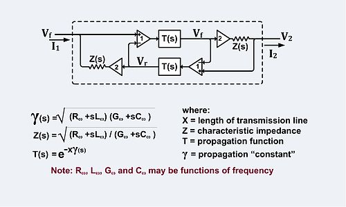Equivalent circuit of a transmission line described by the Telegrapher's equations.

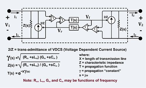Solutions of the Telegrapher's Equations as Components in the Equivalent Circuit of a Balanced Transmission Line Two-Port Implementation.

The solutions of the telegrapher's equations can be inserted directly into a circuit as components. The circuit in the left figure implements the solutions of the telegrapher's equations.^[3]

The right hand circuit is derived from the left hand circuit by source transformations.^[4] It also implements the solutions of the telegrapher's equations.

The solution of the telegrapher's equations can be expressed as an ABCD type Two-port network with the following defining equations^[5]

$V_1 = V_2 cosh ( \gamma x) + I_2 Z sinh (\gamma x) \,$

$I_1 = V_2 \frac{1}{Z} sinh (\gamma x) + I_2 cosh(\gamma x). \,$

The symbols: $E_s, E_L, I_s, I_L, l \,$ in the source book have been replaced by the symbols :$V_1, V_2, I_1, I_2, x \,$ in the preceding two equations.

The ABCD type two-port gives $V_1 \,$ and $I_1 \,$ as functions of $V_2 \,$ and $I_2 \,$. Both of the circuits above, when solved for $V_1 \,$ and $I_1 \,$ as functions of $V_2 \,$ and $I_2 \,$ yield exactly the same equations.

In the right hand circuit, all voltages except the port voltages are with respect to ground and the differential amplifiers have unshown connections to ground. An example of a transmission line modeled by this circuit would be a balanced transmission line such as a telephone line. The impedances Z(s), the voltage dependent current sources (VDCSs) and the difference amplifiers (the triangle with the number "1") account for the interaction of the transmission line with the external circuit. The T(s) blocks account for delay, attenuation, dispersion and whatever happens to the signal in transit. One of the T(s) blocks carries the forward wave and the other carries the backward wave. The circuit, as depicted, is fully symmetric, although it is not drawn that way. The circuit depicted is equivalent to a transmission line connected from $V_1 \,$ to $V_2 \,$ in the sense that $V_1 \,$, $V_2 \,$, $I_1 \,$ and $I_2 \,$ would be same whether this circuit or an actual transmission line was connected between $V_1 \,$ and $V_2 \,$. There is no implication that there are actually amplifiers inside the transmission line.

Every two-wire or balanced transmission line has an implicit (or in some cases explicit) third wire which may be called shield, sheath, common, Earth or ground. So every two-wire balanced transmission line has two modes which are nominally called the differential and common modes. The circuit shown on the right only models the differential mode.

In the left hand circuit, the voltage doublers, the difference amplifiers and impedances Z(s) account for the interaction of the transmission line with the external circuit. This circuit, as depicted, is also fully symmetric, and also not drawn that way. This circuit is a useful equivalent for an unbalanced transmission line like a coaxial cable or a micro strip line.

These are not the only possible equivalent circuits.

See also

Distributed element model Electric power transmission Heaviside condition Longitudinal electromagnetic wave Lumped components Propagation velocity

Radio frequency power transmission Smith chart, a graphical method to solve transmission line equations Standing wave Time domain reflectometer Transverse electromagnetic wave

References

Part of this article was derived from Federal Standard 1037C.

1. ^ Ernst Weber and Frederik Nebeker, The Evolution of Electrical Engineering, IEEE Press, Piscataway, New Jersey USA, 1994 ISBN 0-7803-1066-7
2. ^ Syed V. Ahamed, Victor B. Lawrence, Design and engineering of intelligent communication systems, pp.130-131, Springer, 1997 ISBN 079239870X.
3. ^ McCammon, Roy, SPICE Simulation of Transmission Lines by the Telegrapher's Method, http://i.cmpnet.com/rfdesignline/2010/06/C0580Pt1edited.pdf, retrieved 22 Oct 2010 
4. ^ William H. Hayt (1971). Engineering Circuit Analysis (second ed.). New York, NY: McGraw-Hill. ISBN 070273820. , pp. 73-77
5. ^ John J. Karakash (1950). Transmission Lines and Filter Networks (First ed.). New York, NY: Macmillan. , p. 44

• Steinmetz, Charles Proteus (August 27, 1898), "The Natural Period of a Transmission Line and the Frequency of lightning Discharge Therefrom", The Electrical World: 203–205 
• Grant, I. S.; Phillips, W. R., Electromagnetism (2nd ed.), John Wiley, ISBN 0-471-92712-0 
• Ulaby, F. T., Fundamentals of Applied Electromagnetics (2004 media ed.), Prentice Hall, ISBN 0-13-185089-X 
• "Chapter 17", Radio communication handbook, Radio Society of Great Britain, 1982, pp. 20, ISBN 0-900612-58-4 
• Naredo, J. L.; Soudack, A. C.; Marti, J. R. (Jan 1995), "Simulation of transients on transmission lines with corona via the method of characteristics", IEE Proceedings. Generation, Transmission and Distribution. (Morelos: Institution of Electrical Engineers) 142 (1), ISSN 1350-2360 

External articles and further reading

• Annual Dinner of the Institute at the Waldorf-Astoria. Transactions of the American Institute of Electrical Engineers, New York, January 13, 1902. (Honoring of Guglielmo Marconi, January 13, 1902)
• Avant! software, Using Transmission Line Equations and Parameters. Star-Hspice Manual, June 2001.
• Cornille, P, On the propagation of inhomogeneous waves. J. Phys. D: Appl. Phys. 23, February 14, 1990. (Concept of inhomogeneous waves propagation — Show the importance of the telegrapher's equation with Heaviside's condition.)
• Farlow, S.J., Partial differential equations for scientists and engineers. J. Wiley and Sons, 1982, p. 126. ISBN 0-471-08639-8.
• Kupershmidt, Boris A., Remarks on random evolutions in Hamiltonian representation. Math-ph/9810020. J. Nonlinear Math. Phys. 5 (1998), no. 4, 383-395.
• Pupin, M., U.S. Patent 1,541,845, Electrical wave transmission.
• Transmission line matching. EIE403: High Frequency Circuit Design. Department of Electronic and Information Engineering, Hong Kong Polytechnic University. (PDF format)
• Wilson, B. (2005, October 19). Telegrapher's Equations. Connexions.
• John Greaton Wöhlbier, ""Fundamental Equation" and "Transforming the Telegrapher's Equations". Modeling and Analysis of a Traveling Wave Under Multitone Excitation.
• Agilent Technologies. Educational Resources. Wave Propagation along a Transmission Line. Edutactional Java Applet.
• Qian, C., Impedance matching with adjustable segmented transmission line. J. Mag. Reson. 199 (2009), 104-110.

External links

• Transmission Line Parameter Calculator
• Interactive applets on transmission lines
• SPICE Simulation of Transmission Lines