Latin hypercube sampling

Latin hypercube sampling (LHS) is a statistical method for generating a distribution of plausible collections of parameter values from a multidimensional distribution. The sampling method is often applied in uncertainty analysis.

The technique was first described by McKay in 1979.^[1] It was further elaborated by Ronald L. Iman, and others^[2] in 1981. Detailed computer codes and manuals were later published.^[3]

In the context of statistical sampling, a square grid containing sample positions is a Latin square if (and only if) there is only one sample in each row and each column. A Latin hypercube is the generalisation of this concept to an arbitrary number of dimensions, whereby each sample is the only one in each axis-aligned hyperplane containing it.

When sampling a function of N variables, the range of each variable is divided into M equally probable intervals. M sample points are then placed to satisfy the Latin hypercube requirements; note that this forces the number of divisions, M, to be equal for each variable. Also note that this sampling scheme does not require more samples for more dimensions (variables); this independence is one of the main advantages of this sampling scheme. Another advantage is that random samples can be taken one at a time, remembering which samples were taken so far.

The maximum number of combinations for a Latin Hypercube of M divisions and N variables (i.e., dimensions) can be computed with the following formula:

$\left(\prod_{n=0}^{M-1} (M-n)\right)^{N-1} = (M!)^{N-1}$

For example, a Latin hypercube of M = 4 divisions with N = 2 variables (i.e., a square) will have 24 possible combinations. A Latin hypercube of M = 4 divisions with N = 3 variables (i.e., a cube) will have 576 possible combinations.

Orthogonal sampling adds the requirement that the entire sample space must be sampled evenly. Although more efficient, orthogonal sampling strategy is more difficult to implement since all random samples must be generated simultaneously.

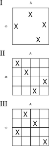
In two dimensions the difference between random sampling, Latin Hypercube sampling and orthogonal sampling can be explained as follows:

1. In random sampling new sample points are generated without taking into account the previously generated sample points. One does thus not necessarily need to know beforehand how many sample points are needed.
2. In Latin Hypercube sampling one must first decide how many sample points to use and for each sample point remember in which row and column the sample point was taken.
3. In Orthogonal Sampling, the sample space is divided into equally probable subspaces, the figure above showing four subspaces. All sample points are then chosen simultaneously making sure that the total ensemble of sample points is a Latin Hypercube sample and that each subspace is sampled with the same density.

Thus, orthogonal sampling ensures that the ensemble of random numbers is a very good representative of the real variability, LHS ensures that the ensemble of random numbers is representative of the real variability whereas traditional random sampling (sometimes called brute force) is just an ensemble of random numbers without any guarantees.

References

1. ^ McKay, M.D.; Beckman, R.J.; Conover, W.J. (May 1979). "A Comparison of Three Methods for Selecting Values of Input Variables in the Analysis of Output from a Computer Code" (JSTOR Abstract). Technometrics (American Statistical Association) 21 (2): 239–245. doi:10.2307/1268522. ISSN 0040-1706. JSTOR 1268522. OSTI 5236110. 
2. ^ Iman, R.L.; Helton, J.C.; and Campbell, J.E. (1981). "An approach to sensitivity analysis of computer models, Part 1. Introduction, input variable selection and preliminary variable assessment". Journal of Quality Technology 13 (3): 174–183. 
3. ^ Iman, R.L.; Davenport, J.M. ; Zeigler, D.K. (1980). Latin hypercube sampling (program user's guide). OSTI 5571631. 

Further reading

• Tang, B. (1993). "Orthogonal Array-Based Latin Hypercubes". Journal of the American Statistical Association 88 (424): 1392–1397. doi:10.2307/2291282. JSTOR 2291282. 
• Owen, A.B. (1992). "Orthogonal arrays for computer experiments, integration and visualization". Statistica Sinica 2: 439–452. 
• Ye, K.Q. (1998). "Orthogonal column Latin hypercubes and their application in computer experiments". Journal of the American Statistical Association 93 (444): 1430–1439. doi:10.2307/2670057. JSTOR 2670057.