Trend estimation

Trend estimation is a statistical technique to aid interpretation of data. When a series of measurements of a process are treated as a time series, trend estimation can be used to make and justify statements about tendencies in the data. By using trend estimation it is possible to construct a model which is independent of anything known about the nature of the process of an incompletely understood system (for example, physical, economic, or other system). This model can then be used to describe the behaviour of the observed data.

In particular, it may be useful to determine if measurements exhibit an increasing or decreasing trend which is statistically distinguished from random behaviour. Some examples are: determining the trend of the daily average temperatures at a given location, from winter to summer; or the trend in a global temperature series over the last 100 years. In the latter case, issues of homogeneity are important (for example, about whether the series is equally reliable throughout its length).

Fitting a trend: least-squares

Given a set of data and the desire to produce some kind of "model" of those data (model, in this case, meaning a function fitted through the data), there are a variety of functions that can be chosen for the fit. However, if there is no prior understanding of the data, then the simplest function to fit is a straight line. However, doing so makes many assumptions about the nature of the data (which depend on the method used). Whether the resulting line actually "means" anything needs to be carefully assessed. Just because a mathematical method produces a straight line does not mean it represents a real "trend" or reflects the relationship of the two variables.

Once it has been decided to fit a straight line, there are various ways to do so, but the most usual choice is a least-squares fit. This method minimises the sum of the squared errors in the y variable. See least squares. The method assumes that the error or uncertainly in the x values is much smaller than the y errors. If this is not the case the answer will be wrong. It can be shown that as x error increases the slope will be increasingly underestimated. In this case more complex techniques need to be used.

Given a set of points in time t, and data values y_t observed for those points in time, values of a and b are chosen so that

$\sum_t \left\{[(at + b) - y_t]^2\right\}$

is minimised. Here at + b is the trend line, so the sum of squared deviations from the trend line is what is being minimised. This can always be done in closed form since this is a case of simple linear regression.

For the rest of this article, "trend" will mean the slope of the least squares line, since this is a common convention.

Trends in random data

Before considering trends in real data, it is useful to understand trends in random data.

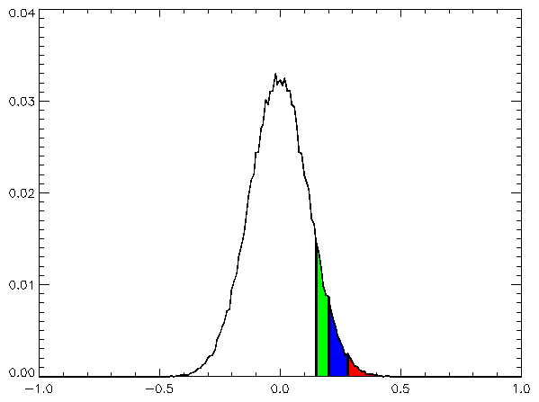
Red shaded values are greater than 99% of the rest; blue, 95%; green, 90%. In this case, the V values discussed in the text for (one-sided) 95% confidence is seen to be 0.2.

If a series is analysed which is known to be random – fair dice falls; or computer-generated pseudo-random numbers – and a trend line is fitted through the data, the chances of a truly zero estimated trend are negligible. But the trend would probably be expected to be "small". If an individual series of observations from simulations is described as having a given degree of noise, and a given length (say, 100 points), a large number of such simulated series (say, 100,000 series) can be generated. These 100,000 series can then be analysed individually to calculate the trends in each series, and these results establish empirically a distribution of trends that are to be expected from such random data – see diagram. Such a distribution will be normal (central limit theorem except in pathological cases, since – in a slightly non-obvious way of thinking about it – the trend is a linear combination of the y_t) and, if the series genuinely is random, centered on zero. A level of statistical certainty, S, may now be selected – 95% confidence is typical; 99% would be stricter, 90% rather looser – and the following question can be asked: what value, V, do we have to choose so that S% of trends are within −V to +V?

In the above discussion the distribution of trends was calculated empirically, from a large number of trials. In simple cases (normally distributed random noise being a classic) the distribution of trends can be calculated exactly without simulation.

Suppose the actual series of observed data that needs to be analysed has approximately the same variance properties as the random series used in the above empirical investigation. It is not known in advance whether the observed series "really" has a trend in it, but the trend, a, can be estimated and a determination can be made of whether this value lies within the range −V to +V. If the estimated value of a does lie in this range, it can be said that, at degree of certainty S, any trend in the data cannot be distinguished from random noise. That is, one cannot reject the null hypothesis of no trend.

However, note that whatever value of S we choose, then a given fraction, 1 − S, of truly random series will be declared (falsely, by construction) to have a significant trend. Conversely, a certain fraction of series that "really" have a trend will not be declared to have a trend.

The above procedure can be turned into a well-established statistical procedure, called a permutation test. For this, the set of 100,000 generated series would be replaced by 100,000 series constructed from the observed data series by, for each generated series, creating a random rearrangement in time of the original series: clearly such constricted series would be "trend-free".

Data as trend plus noise

To analyse a (time) series of data, we assume that it may be represented as trend plus noise:

$y_t = at + b + e_t\,$

where a and b are unknown constants and the e's are randomly distributed errors. If one can reject the null hypothesis that the errors are non-stationary, then the non-stationary series {y_t } is called trend stationary. The least squares method assumes the errors to be independently distributed with a normal distribution. If this is not the case the result may be inaccurate. It is simplest if the e's all have the same distribution, but if not (if some have higher variance, meaning that those data points are effectively less certain) then this can be taken into account during the least squares fitting, by weighting each point by the inverse of the variance of that point.

In most cases, where only a single time series exists to be analysed, the variance of the e's is estimated by fitting a trend, thus allowing at + b to be subtracted from the data y_t (thus detrending the data) and leaving the residuals e_t as the detrended data, and calculating the variance of the e_t's from the residuals — this is often the only way of estimating the variance of the e_t's.

One particular special case of great interest, the (global) temperature time series, is known not to be homogeneous in time: apart from anything else, the number of weather observations has (generally) increased with time, and thus the error associated with estimating the global temperature from a limited set of observations has decreased with time. In fitting a trend to this data, this can be taken into account, as described above. Though many people do attempt to fit a "trend" to climate data the climate trend is clearly not a straight line and the idea of attributing a straight line is not mathematically correct because the assumptions of the method are not valid in this context.

Once we know the "noise" of the series, we can then assess the significance of the trend by making the null hypothesis that the trend, a, is not significantly different from 0. From the above discussion of trends in random data with known variance, we know the distribution of trends to be expected from random (trendless) data. If the calculated trend, a, is larger than the value, V, then the trend is deemed significantly different from zero at significance level S.

The use of a linear trend line has been the subject of criticism, leading to a search for alternative approaches to avoid its use in model estimation. One of the alternative approaches involves unit root tests and the cointegration technique in econometric studies.

The estimated coefficient associated with a linear time trend variable is interpreted as a measure of the impact of a number of unknown or known but unmeasurable factors on the dependent variable over one unit of time. Strictly speaking, that interpretation is applicable for the estimation time frame only. Outside that time frame, one does not know how those unmeasurable factors behave both qualitatively and quantitatively. Furthermore, the linearity of the time trend poses many questions:

(i) Why should it be linear?

(ii) If the trend is non-linear then under what conditions does its inclusion influence the magnitude as well as the statistical significance of the estimates of other parameters in the model?

(iii) The inclusion of a linear time trend in a model precludes by assumption the presence of fluctuations in the tendencies of the dependent variable over time; is this necessarily valid in a particular context?

(iv) And, does a spurious relationship exist in the model because an underlying causative variable is itself time-trending?

Research results of mathematicians, statisticians, econometricians, and economists have been published in response to those questions. For example, detailed notes on the meaning of linear time trends in regression model are given in Cameron (2005)^[1]; Granger, Engle and many other econometricians have written on stationarity, unit root testing, co-integration and related issues (a summary of some of the works in this area can be found in an information paper^[2] by the Royal Swedish Academy of Sciences (2003); and Ho-Trieu & Tucker (1990) have written on logarithmic time trends^[3] with results indicating linear time trends are special cases of business cycles ^[4].

Noisy time series, and an example

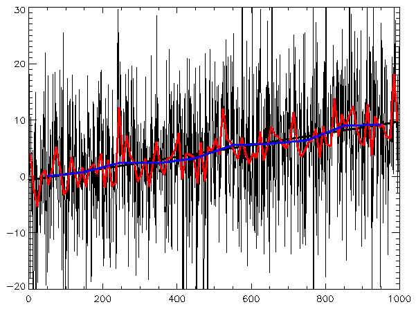
It is harder to see a trend in a noisy time series. For example, if the true series is 0, 1, 2, 3 all plus some independent normally distributed "noise" e of standard deviation E, and we have a sample series of length 50, then if E = 0.1 the trend will be obvious; if E = 100 the trend will probably be visible; but if E = 10000 the trend will be buried in the noise.

If we consider a concrete example, the global surface temperature record of the past 140 years as presented by the IPCC: ^[5] then the interannual variation is about 0.2°C and the trend about 0.6°C over 140 years, with 95% confidence limits of 0.2°C (by coincidence, about the same value as the interannual variation). Hence the trend is statistically different from 0.

Goodness of fit (R-squared) and trend

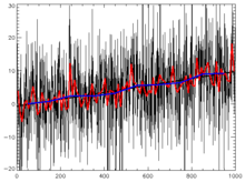Illustration of the variation of r² with filtering while fit remains the same

The least-squares fitting process produces a value – r-squared (r²) – which is the square of the residuals of the data after the fit. It says what fraction of the variance of the data is explained by the fitted trend line. It does not relate to the statistical significance of the trend line (see graph); statistical significance of the trend is determined by its t-statistic. A noisy series can have a very low r² value but a very high significance in a test for the presence of trend. Often, filtering a series increases r² while making little difference to the fitted trend or significance. In a method for identifying a statistically meaningful trend, only filtered or unfiltered series with r² values exceeding 0.65 are counted as positive test results.

Real data need more complicated models

Thus far the data have been assumed to consist of the trend plus noise, with the noise at each data point being independent and identically-distributed random variables and to have a normal distribution. Real data (for example climate data) may not fulfill these criteria. This is important, as it makes an enormous difference to the ease with which the statistics can be analysed so as to extract maximum information from the data series. If there are other non-linear effects that have a correlation to the independent variable (such as a super-exponential increase in GHG or cyclic influences), the use of least-squares estimation of the trend is not valid. Also where the variations are significantly larger than the resulting straight line trend, the choice of start and end points can significantly change the result. That is , mathematically, the result is inconsistent. Statistical inferences (tests for the presence of trend, confidence intervals for the trend, etc.) are invalid unless departures from the standard assumptions are properly accounted for, for example as follows:

• Dependence: autocorrelated time series might be modeled using autoregressive moving average models.

• Non-constant variance: in the simplest cases weighted least squares might be used.

• Non-normal distribution for errors: in the simplest cases a generalised linear model might be applicable.

• Unit root: taking first differences of the data

See also

• Extrapolation
• Forecasting
• Prediction interval
• Regression analysis

Notes

1. ^ . http://highered.mcgraw-hill.com/sites/dl/free/0077104285/160071/Chapter_7.pdf. 
2. ^ . http://www.kva.se/Documents/Priser/Nobel/2003/sciback_ek_en_03.pdf. 
3. ^ . http://ageconsearch.umn.edu/bitstream/12288/1/58010089.pdf. 
4. ^ . http://ageconsearch.umn.edu/bitstream/12288/1/58010089.pdf. 
5. ^ . http://www.grida.no/publications/other/ipcc_tar/?src=/climate/ipcc_tar/wg1/figspm-1.htm. 

References

• Bianchi M., Boyle M., Hollingsworth D. (1999), "A comparison of methods for trend estimation", Applied Economics Letters, 6(2): 103–109.

• Cameron S. (2005), Econometrics, Chapter 7, McGraw Hill Higher Education.

• Chatfield, C. (1993), "Calculating Interval Forecasts", Journal of Business and Economic Statistics, 11(2): 121–135.

• Ho-Trieu N.L., Tucker J. (1990), Another note on the use of a logarithmic time trend, Review of Marketing and Agricultural Economics, 58(1): 89–90.

• Kungl. Vetenskapsakademien (The Royal Swedish Academy of Sciences) (2003), Time-series econometrics: Cointegration and autoregressive conditional heteroskedasticity, Advanced information on the Bank of Sweden Prize in Economic Sciences in Memory of Alfred Nobel.