- Algorithm
-
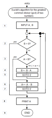 Flow chart of an algorithm (Euclid's algorithm) for calculating the greatest common divisor (g.c.d.) of two numbers a and b in locations named A and B. The algorithm proceeds by successive subtractions in two loops: IF the test B ≤ A yields "yes" (or true) (more accurately the number b in location B is less than or equal to the number a in location A) THEN the algorithm specifies B ← B − A (meaning the number b − a replaces the old b). Similarly IF A > B THEN A ← A − B. The process terminates when (the contents of) B is 0, yielding the g.c.d. in A. (Algorithm derived from Scott 2009:13; symbols and drawing style from Tausworthe 1977).
In mathematics and computer science, an algorithm
 i/ˈælɡərɪðəm/ is an effective method expressed as a finite list[1] of well-defined instructions[2] for calculating a function.[3] Algorithms are used for calculation, data processing, and automated reasoning. In simple words an algorithm is a step-by-step procedure for calculations.
Starting from an initial state and initial input (perhaps empty),[4] the instructions describe a computation that, when executed, will proceed through a finite [5] number of well-defined successive states, eventually producing "output"[6] and terminating at a final ending state. The transition from one state to the next is not necessarily deterministic; some algorithms, known as randomized algorithms, incorporate random input.[7]
A partial formalization of the concept began with attempts to solve the Entscheidungsproblem (the "decision problem") posed by David Hilbert in 1928. Subsequent formalizations were framed as attempts to define "effective calculability"[8] or "effective method";[9] those formalizations included the Gödel–Herbrand–Kleene recursive functions of 1930, 1934 and 1935, Alonzo Church's lambda calculus of 1936, Emil Post's "Formulation 1" of 1936, and Alan Turing's Turing machines of 1936–7 and 1939. Giving a formal definition of algorithms, corresponding to the intuitive notion, remains a challenging problem.[10]
Why algorithms are necessary: an informal definition
- For a detailed presentation of the various points of view around the definition of "algorithm" see Algorithm characterizations. For examples of simple addition algorithms specified in the detailed manner described in Algorithm characterizations, see Algorithm examples.
While there is no generally accepted formal definition of "algorithm," an informal definition could be "a set of rules that precisely defines a sequence of operations."[11] For some people, a program is only an algorithm if it stops eventually; for others, a program is only an algorithm if it stops before a given number of calculation steps.[12]
A prototypical example of an algorithm is Euclid's algorithm to determine the maximum common divisor of two integers; an example (there are others) is described by the flow chart above and as an example in a later section.
Boolos & Jeffrey (1974, 1999) offer an informal meaning of the word in the following quotation:
No human being can write fast enough, or long enough, or small enough† ( †"smaller and smaller without limit ...you'd be trying to write on molecules, on atoms, on electrons") to list all members of an enumerably infinite set by writing out their names, one after another, in some notation. But humans can do something equally useful, in the case of certain enumerably infinite sets: They can give explicit instructions for determining the nth member of the set, for arbitrary finite n. Such instructions are to be given quite explicitly, in a form in which they could be followed by a computing machine, or by a human who is capable of carrying out only very elementary operations on symbols.[13]
The term "enumerably infinite" means "countable using integers perhaps extending to infinity." Thus Boolos and Jeffrey are saying that an algorithm implies instructions for a process that "creates" output integers from an arbitrary "input" integer or integers that, in theory, can be chosen from 0 to infinity. Thus an algorithm can be an algebraic equation such as y = m + n—two arbitrary "input variables" m and n that produce an output y. But various authors' attempts to define the notion (see more at Algorithm characterizations) indicate that the word implies much more than this, something on the order of (for the addition example):
- Precise instructions (in language understood by "the computer")[14] for a fast, efficient, "good"[15] process that specifies the "moves" of "the computer" (machine or human, equipped with the necessary internally contained information and capabilities)[16] to find, decode, and then process arbitrary input integers/symbols m and n, symbols + and = ... and "effectively"[17] produce, in a "reasonable" time,[18] output-integer y at a specified place and in a specified format.
The concept of algorithm is also used to define the notion of decidability. That notion is central for explaining how formal systems come into being starting from a small set of axioms and rules. In logic, the time that an algorithm requires to complete cannot be measured, as it is not apparently related with our customary physical dimension. From such uncertainties, that characterize ongoing work, stems the unavailability of a definition of algorithm that suits both concrete (in some sense) and abstract usage of the term.
Formalization
Algorithms are essential to the way computers process data. Many computer programs contain algorithms that detail the specific instructions a computer should perform (in a specific order) to carry out a specified task, such as calculating employees' paychecks or printing students' report cards. Thus, an algorithm can be considered to be any sequence of operations that can be simulated by a Turing-complete system. Authors who assert this thesis include Minsky (1967), Savage (1987) and Gurevich (2000):
Minsky: "But we will also maintain, with Turing . . . that any procedure which could "naturally" be called effective, can in fact be realized by a (simple) machine. Although this may seem extreme, the arguments . . . in its favor are hard to refute".[19]
Gurevich: "...Turing's informal argument in favor of his thesis justifies a stronger thesis: every algorithm can be simulated by a Turing machine ... according to Savage [1987], an algorithm is a computational process defined by a Turing machine".[20]
Typically, when an algorithm is associated with processing information, data is read from an input source, written to an output device, and/or stored for further processing. Stored data is regarded as part of the internal state of the entity performing the algorithm. In practice, the state is stored in one or more data structures.
For some such computational process, the algorithm must be rigorously defined: specified in the way it applies in all possible circumstances that could arise. That is, any conditional steps must be systematically dealt with, case-by-case; the criteria for each case must be clear (and computable).
Because an algorithm is a precise list of precise steps, the order of computation will always be critical to the functioning of the algorithm. Instructions are usually assumed to be listed explicitly, and are described as starting "from the top" and going "down to the bottom", an idea that is described more formally by flow of control.
So far, this discussion of the formalization of an algorithm has assumed the premises of imperative programming. This is the most common conception, and it attempts to describe a task in discrete, "mechanical" means. Unique to this conception of formalized algorithms is the assignment operation, setting the value of a variable. It derives from the intuition of "memory" as a scratchpad. There is an example below of such an assignment.
For some alternate conceptions of what constitutes an algorithm see functional programming and logic programming.
Expressing algorithms
Algorithms can be expressed in many kinds of notation, including natural languages, pseudocode, flowcharts, programming languages or control tables (processed by interpreters). Natural language expressions of algorithms tend to be verbose and ambiguous, and are rarely used for complex or technical algorithms. Pseudocode, flowcharts and control tables are structured ways to express algorithms that avoid many of the ambiguities common in natural language statements. Programming languages are primarily intended for expressing algorithms in a form that can be executed by a computer, but are often used as a way to define or document algorithms.
There is a wide variety of representations possible and one can express a given Turing machine program as a sequence of machine tables (see more at finite state machine and state transition table), as flowcharts (see more at state diagram), or as a form of rudimentary machine code or assembly code called "sets of quadruples" (see more at Turing machine).
Representations of algorithms can be classed into three accepted levels of Turing machine description:[21]
- 1 High-level description:
-
- "...prose to describe an algorithm, ignoring the implementation details. At this level we do not need to mention how the machine manages its tape or head."
- 2 Implementation description:
-
- "...prose used to define the way the Turing machine uses its head and the way that it stores data on its tape. At this level we do not give details of states or transition function."
- 3 Formal description:
-
- Most detailed, "lowest level", gives the Turing machine's "state table".
- For an example of the simple algorithm "Add m+n" described in all three levels see Algorithm examples.
Implementation
Most algorithms are intended to be implemented as computer programs. However, algorithms are also implemented by other means, such as in a biological neural network (for example, the human brain implementing arithmetic or an insect looking for food), in an electrical circuit, or in a mechanical device.
Computer algorithms
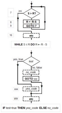 Flowchart examples of the canonical Böhm-Jacopini structures: the SEQUENCE (rectangles descending the page), the WHILE-DO and the IF-THEN-ELSE. The three structures are made of the primitive conditional GOTO (IF test=true THEN GOTO step xxx) (a diamond), the unconditional GOTO (rectangle), various assignment operators (rectangle), and HALT (rectangle). Nesting of these structures inside assignment-blocks result in complex diagrams (cf Tausworthe 1977:100,114).
In computer systems, an algorithm is basically an instance of logic written in software by software developers to be effective for the intended "target" computer(s), in order for the target machines to produce output from given input (perhaps null).
"Elegant" (compact) programs, "good" (fast) programs : The notion of "simplicity and elegance" appears informally in Knuth and precisely in Chaitin:
- Knuth: ". . .we want good algorithms in some loosely defined aesthetic sense. One criterion . . . is the length of time taken to perform the algorithm . . .. Other criteria are adaptability of the algorithm to computers, its simplicity and elegance, etc"[22]
- Chaitin: " . . . a program is 'elegant,' by which I mean that it's the smallest possible program for producing the output that it does"[23]
Chaitin prefaces his definition with: "I'll show you can't prove that a program is 'elegant'"—such a proof would solve the Halting problem (ibid).
Algorithm versus function computable by an algorithm: For a given function multiple algorithms may exist. This will be true, even without expanding the available instruction set available to the programmer. Rogers observes that "It is . . . important to distinguish between the notion of algorithm, i.e. procedure and the notion of function computable by algorithm, i.e. mapping yielded by procedure. The same function may have several different algorithms".[24]
Unfortunately there may be a tradeoff between goodness (speed) and elegance (compactness)—an elegant program may take more steps to complete a computation than one less elegant. An example of using Euclid's algorithm will be shown below.
Computers (and computors), models of computation: A computer (or human "computor"[25]) is a restricted type of machine, a "discrete deterministic mechanical device"[26] that blindly follows its instructions.[27] Melzak's and Lambek's primitive models[28] reduced this notion to four elements: (i) discrete, distinguishable locations, (ii) discrete, indistinguishable counters[29] (iii) an agent, and (iv) a list of instructions that are effective relative to the capability of the agent.[30]
Minsky describes a more congenial variation of Lambek's "abacus" model in his "Very Simple Bases for Computability".[31] Minsky's machine proceeds sequentially through its five (or six depending on how one counts) instructions unless either a conditional IF–THEN GOTO or an unconditional GOTO changes program flow out of sequence. Besides HALT, Minsky's machine includes three assignment (replacement, substitution)[32] operations: ZERO (e.g. the contents of location replaced by 0: L ← 0), SUCCESSOR (e.g. L ← L+1), and DECREMENT (e.g. L ← L − 1).[33] Rarely will a programmer have to write "code" with such a limited instruction set. But Minsky shows (as do Melzak and Lambek) that his machine is Turing complete with only four general types of instructions: conditional GOTO, unconditional GOTO, assignment/replacement/substitution, and HALT.[34]
Simulation of an algorithm: computer (computor) language: Knuth advises the reader that "the best way to learn an algorithm is to try it . . . immediately take pen and paper and work through an example".[35] But what about a simulation or execution of the real thing? The programmer must translate the algorithm into a language that the simulator/computer/computor can effectively execute. Stone gives an example of this: when computing the roots of a quadratic equation the computor must know how to take a square root. If they don't then for the algorithm to be effective it must provide a set of rules for extracting a square root.[36]
This means that the programmer must know a "language" that is effective relative to the target computing agent (computer/computor).
But what model should be used for the simulation? Van Emde Boas observes "even if we base complexity theory on abstract instead of concrete machines, arbitrariness of the choice of a model remains. It is at this point that the notion of simulation enters".[37] When speed is being measured, the instruction set matters. For example, the subprogram in Euclid's algorithm to compute the remainder would execute much faster if the programmer had a "modulus" (division) instruction available rather than just subtraction (or worse: just Minsky's "decrement").
Structured programming, canonical structures: Per the Church-Turing thesis any algorithm can be computed by a model known to be Turing complete, and per Minsky's demonstrations Turing completeness requires only four instruction types—conditional GOTO, unconditional GOTO, assignment, HALT. Kemeny and Kurtz observe that while "undisciplined" use of unconditional GOTOs and conditional IF-THEN GOTOs can result in "spaghetti code" a programmer can write structured programs using these instructions; on the other hand "it is also possible, and not too hard, to write badly structured programs in a structured language".[38] Tausworthe augments the three Böhm-Jacopini canonical structures:[39] SEQUENCE, IF-THEN-ELSE, and WHILE-DO, with two more: DO-WHILE and CASE.[40] An additional benefit of a structured program will be one that lends itself to proofs of correctness using mathematical induction.[41]
Canonical flowchart symbols[42]: The graphical aide called a flowchart offers a way to describe and document an algorithm (and a computer program of one). Like program flow of a Minsky machine, a flowchart always starts at the top of a page and proceeds down. Its primary symbols are only 4: the directed arrow showing program flow, the rectangle (SEQUENCE, GOTO), the diamond (IF-THEN-ELSE), and the dot (OR-tie). The Böhm-Jacopini canonical structures are made of these primitive shapes. Sub-structures can "nest" in rectangles but only if a single exit occurs from the superstructure. The symbols and their use to build the canonical structures are shown in the diagram.
Examples
Further information: Algorithm examplesSorting example
 An animation of the quicksort algorithm sorting an array of randomized values. The red bars mark the pivot element; at the start of the animation, the element farthest to the right hand side is chosen as the pivot.
One of the simplest algorithms is to find the largest number in an (unsorted) list of numbers. The solution necessarily requires looking at every number in the list, but only once at each. From this follows a simple algorithm, which can be stated in a high-level description English prose, as:
High-level description:
- Assume the first item is largest.
- Look at each of the remaining items in the list and if it is larger than the largest item so far, make a note of it.
- The last noted item is the largest in the list when the process is complete.
(Quasi-)formal description: Written in prose but much closer to the high-level language of a computer program, the following is the more formal coding of the algorithm in pseudocode or pidgin code:
Algorithm LargestNumber
  Input: A non-empty list of numbers L.
  Output: The largest number in the list L.
largest ← L0 for each item in the list (Length(L)≥1), do if the item > largest, then largest ← the item return largest- "←" is a loose shorthand for "changes to". For instance, "largest ← item" means that the value of largest changes to the value of item.
- "return" terminates the algorithm and outputs the value that follows.
Euclid’s algorithm
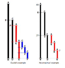 The example-diagram of Euclid's algorithm from T.L. Heath 1908 with more detail added. Euclid does not go beyond a third measuring and gives no numerical examples. Nicomachus gives the example of 49 and 21: "I subtract the less from the greater; 28 is left; then again I subtract from this the same 21 (for this is possible); 7 is left; I subtact this from 21, 14 is left; from which I again subtract 7 (for this is possible); 7 will be left, but 7 cannot be subtracted from 7." Heath comments that "The last phrase is curious, but the meaning of it is obvious enough, as also the meaning of the phrase about ending "at one and the same number"(Heath 1908:300).
Euclid’s algorithm appears as Proposition II in Book VII ("Elementary Number Theory") of his Elements.[43] Euclid poses the problem: "Given two numbers not prime to one another, to find their greatest common measure". He defines "A number [to be] a multitude composed of units": a counting number, a positive integer not including 0. And to "measure" is to place a shorter measuring length s successively (q times) along longer length l until the remaining portion r is less than the shorter length s.[44] In modern words, remainder r = l − q*s, q being the quotient, or remainder r is the "modulus", the integer-fractional part left over after the division.[45]
For Euclid’s method to succeed, the starting lengths must satisfy two requirements: (i) the lengths must not be 0, AND (ii) the subtraction must be “proper”, a test must guarantee that the smaller of the two numbers is subtracted from the larger (alternately, the two can be equal so their subtraction yields 0).
Euclid's original proof adds a third: the two lengths are not prime to one another. Euclid stipulated this so that he could construct a reductio ad absurdum proof that the two numbers' common measure is in fact the greatest.[46] While Nicomachus' algorithm is the same as Euclid's, when the numbers are prime to one another it yields the number "1" for their common measure. So to be precise the following is really Nicomachus' algorithm.
Example
 A graphical expression on Euclid's algorithm using example with 1599 and 650.
Example of 1599 and 650 :
Step 1 1599 = 650*2 + 299 Step 2 650 = 299*2 + 52 Step 3 299 = 52*5 + 39 Step 4 52 = 39*1 + 13 Step 5 39 = 13*3 + 0 Computer (computor) language for Euclid's algorithm
Only a few instruction types are required to execute Euclid's algorithm—some logical tests (conditional GOTO), unconditional GOTO, assignment (replacement), and subtraction.
- A location is symbolized by upper case letter(s), e.g. S, A, etc.
- The varying quantity (number) in a location will be written in lower case letter(s) and (usually) associated with the location's name. For example, location L at the start might contain the number l = 3009.
An inelegant program for Euclid's algorithm
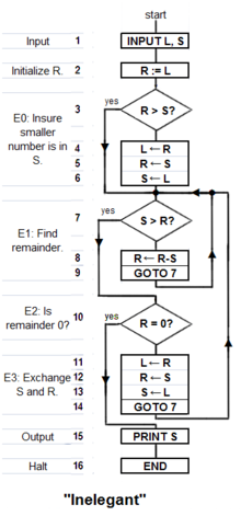 "Inelegant" is a translation of Knuth's version of the algorithm with a subtraction-based remainder-loop replacing his use of division (or a "modulus" instruction). Derived from Knuth 1973:2–4. Depending on the two numbers "Inelegant" may compute the g.c.d. in fewer steps than "Elegant".
The following algorithm is framed as Knuth's 4-step version of Euclid's and Nichomachus', but rather than using division to find the remainder it uses successive subtractions of the shorter length s from the remaining length r until r is less than s. The high-level description, shown in boldface, is adapted from Knuth 1973:2–4:
INPUT:
- 1 [Into two locations L and S put the numbers l and s that represent the two lengths]: INPUT L, S
- 2 [Initialize R: make the remaining length r equal to the starting/initial/input length l] R ← L
E0: [Insure r ≥ s.]
- 3 [Insure the smaller of the two numbers is in S and the larger in R]: IF R > S THEN the contents of L is the larger number so skip over the exchange-steps 4, 5 and 6: GOTO step 6 ELSE swap the contents of R and S.]
- 4 L ← R (this first step is redundant, but will be useful for later discussion).
- 5 R ← S
- 6 S ← L
E1:[Find remainder]: Until the remaining length r in R is less than the shorter length s in S, repeatedly subtract the measuring number s in S from the remaining length r in R.
- 7 IF S > R THEN done measuring so GOTO 10 ELSE measure again,
- 8 R ← R − S
- 9 [Remainder-loop]: GOTO 7.
E2: [Is the remainder 0?]: EITHER (i) the last measure was exact and the remainder in R is 0 program can halt, OR (ii) the algorithm must continue: the last measure left a remainder in R less than measuring number in S.
- 10 IF R = 0 then done so GOTO step 15 ELSE continue to step 11,
E3: [Interchange s and r ]: The nut of Euclid's algorithm. Use remainder r to measure what was previously smaller number s:; L serves as a temporary location.
- 11 L ← R
- 12 R ← S
- 13 S ← L
- 14 [Repeat the measuring process]: GOTO 7
OUTPUT:
- 15 [Done. S contains the greatest common divisor]: PRINT S
DONE:
- 16 HALT, END, STOP.
An elegant program for Euclid's algorithm
The following version of Euclid's algorithm requires only 6 core instructions to do what 13 are required to do by "Inelegant"; worse, "Inelegant" requires more types of instructions. The flowchart of "Elegant" can be found at the top of this article. In the (unstructured) Basic language the steps are numbered, and the instruction LET [ ] = [ ] is the assignment instruction symbolized by ←.
   5 REM Euclid's algorithm for greatest common divisor
   6 PRINT "Type two integers greater than 0"
   10 INPUT A,B
   20 IF B=0 THEN GOTO 80
   30 IF A > B THEN GOTO 60
   40 LET B=B-A
   50 GOTO 20
   60 LET A=A-B
   70 GOTO 20
   80 PRINT A
   90 END
How "Elegant" works: In place of an outer "Euclid loop", "Elegant" shifts back and forth between two "co-loops", an A > B loop that computes A ← A − B, and a B ≤ A loop that computes B ← B − A. This works because, when at last the minuend M is less than or equal to the subtrahend S ( Difference = Minuend − Subtrahend), the minuend can become s (the new measuring length) and the subtrahend can become the new r (the length to be measured); in other words the "sense" of the subtraction reverses.
Testing the Euclid algorithms
Does an algorithm do what its author wants it to do? A few test cases usually suffice to confirm core functionality. One source[47] uses 3009 and 884. Knuth suggested 40902, 24140. Another interesting case is the two relatively-prime numbers 14157 and 5950.
But exceptional cases must be identified and tested. Will "Inelegant" perform properly when R > S, S > R, R = S? Ditto for "Elegant": B > A, A > B, A = B? (Yes to all). What happens when one number is zero, both numbers are zero? ("Inelegant" computes forever in all cases; "Elegant" computes forever when A = 0.) What happens if negative numbers are entered? Fractional numbers? If the input numbers, i.e. the domain of the function computed by the algorithm/program, is to include only positive integers including zero, then the failures at zero indicate that the algorithm (and the program that instantiates it) is a partial function rather than a total function. A notable failure due to exceptions is the Ariane V rocket failure.
Proof of program correctness by use of mathematical induction: Knuth demonstrates the application of mathematical induction to an "extended" version of Euclid's algorithm, and he proposes "a general method applicable to proving the validity of any algorithm".[48] Tausworthe proposes that a measure of the complexity of a program be the length of its correctness proof.[49]
Measuring and improving the Euclid algorithms
Elegance (compactness) versus goodness (speed) : With only 6 core instructions, "Elegant" is the clear winner compared to "Inelegant" at 13 instructions. However, "Inelegant" is faster (it arrives at HALT in fewer steps). Algorithm analysis[50] indicates why this is the case: "Elegant" does two conditional tests in every subtraction loop, whereas "Inelegant" only does one. As the algorithm (usually) requires many loop-throughs, on average much time is wasted doing a "B = 0?" test that is needed only after the remainder is computed.
Can the algorithms be improved?: Once the programmer judges a program "fit" and "effective"—that is, it computes the function intended by its author—then the question becomes, can it be improved?
The compactness of "Inelegant" can be improved by the elimination of 5 steps. But Chaitin proved that compacting an algorithm cannot be automated by a generalized algorithm;[51] rather, it can only be done heuristically, i.e. by exhaustive search (examples to be found at Busy beaver), trial and error, cleverness, insight, application of inductive reasoning, etc. Observe that steps 4, 5 and 6 are repeated in steps 11, 12 and 13. Comparison with "Elegant" provides a hint that these steps together with steps 2 and 3 can be eliminated. This reduces the number of core instructions from 13 to 8, which makes it "more elegant" than "Elegant" at 9 steps.
The speed of "Elegant" can be improved by moving the B=0? test outside of the two subtraction loops. This change calls for the addition of 3 instructions (B=0?, A=0?, GOTO). Now "Elegant" computes the example-numbers faster; whether for any given A, B and R, S this is always the case would require a detailed analysis.
Algorithmic analysis
Main article: Analysis of algorithmsIt is frequently important to know how much of a particular resource (such as time or storage) is theoretically required for a given algorithm. Methods have been developed for the analysis of algorithms to obtain such quantitative answers (estimates); for example, the sorting algorithm above has a time requirement of O(n), using the big O notation with n as the length of the list. At all times the algorithm only needs to remember two values: the largest number found so far, and its current position in the input list. Therefore it is said to have a space requirement of O(1), if the space required to store the input numbers is not counted, or O(n) if it is counted.
Different algorithms may complete the same task with a different set of instructions in less or more time, space, or 'effort' than others. For example, a binary search algorithm will usually outperform a brute force sequential search when used for table lookups on sorted lists.
Formal versus empirical
Main articles: Empirical algorithmics, Profiling (computer programming), and Program optimizationThe analysis and study of algorithms is a discipline of computer science, and is often practiced abstractly without the use of a specific programming language or implementation. In this sense, algorithm analysis resembles other mathematical disciplines in that it focuses on the underlying properties of the algorithm and not on the specifics of any particular implementation. Usually pseudocode is used for analysis as it is the simplest and most general representation. However, ultimately, most algorithms are usually implemented on particular hardware / software platforms and their algorithmic efficiency is eventually put to the test using real code.
Empirical testing is useful because it may uncover unexpected interactions that affect performance. Benchmarks may be used to compare before/after potential improvements to an algorithm after program optimization.
Classification
There are various ways to classify algorithms, each with its own merits.
By implementation
One way to classify algorithms is by implementation means.
- Recursion or iteration: A recursive algorithm is one that invokes (makes reference to) itself repeatedly until a certain condition matches, which is a method common to functional programming. Iterative algorithms use repetitive constructs like loops and sometimes additional data structures like stacks to solve the given problems. Some problems are naturally suited for one implementation or the other. For example, towers of Hanoi is a well understood in recursive implementation. Every recursive version has an equivalent (but possibly more or less complex) iterative version, and vice versa.
- Logical: An algorithm may be viewed as controlled logical deduction. This notion may be expressed as: Algorithm = logic + control.[52] The logic component expresses the axioms that may be used in the computation and the control component determines the way in which deduction is applied to the axioms. This is the basis for the logic programming paradigm. In pure logic programming languages the control component is fixed and algorithms are specified by supplying only the logic component. The appeal of this approach is the elegant semantics: a change in the axioms has a well-defined change in the algorithm.
- Serial or parallel or distributed: Algorithms are usually discussed with the assumption that computers execute one instruction of an algorithm at a time. Those computers are sometimes called serial computers. An algorithm designed for such an environment is called a serial algorithm, as opposed to parallel algorithms or distributed algorithms. Parallel algorithms take advantage of computer architectures where several processors can work on a problem at the same time, whereas distributed algorithms utilize multiple machines connected with a network. Parallel or distributed algorithms divide the problem into more symmetrical or asymmetrical subproblems and collect the results back together. The resource consumption in such algorithms is not only processor cycles on each processor but also the communication overhead between the processors. Sorting algorithms can be parallelized efficiently, but their communication overhead is expensive. Iterative algorithms are generally parallelizable. Some problems have no parallel algorithms, and are called inherently serial problems.
- Deterministic or non-deterministic: Deterministic algorithms solve the problem with exact decision at every step of the algorithm whereas non-deterministic algorithms solve problems via guessing although typical guesses are made more accurate through the use of heuristics.
- Exact or approximate: While many algorithms reach an exact solution, approximation algorithms seek an approximation that is close to the true solution. Approximation may use either a deterministic or a random strategy. Such algorithms have practical value for many hard problems.
- Quantum algorithm: Quantum algorithm run on a realistic model of quantum computation. The term is usually used for those algorithms which seem inherently quantum, or use some essential feature of quantum computation such as quantum superposition or quantum entanglement.
By design paradigm
Another way of classifying algorithms is by their design methodology or paradigm. There is a certain number of paradigms, each different from the other. Furthermore, each of these categories will include many different types of algorithms. Some commonly found paradigms include:
- Brute-force or exhaustive search. This is the naïve method of trying every possible solution to see which is best.[53]
- Divide and conquer. A divide and conquer algorithm repeatedly reduces an instance of a problem to one or more smaller instances of the same problem (usually recursively) until the instances are small enough to solve easily. One such example of divide and conquer is merge sorting. Sorting can be done on each segment of data after dividing data into segments and sorting of entire data can be obtained in the conquer phase by merging the segments. A simpler variant of divide and conquer is called a decrease and conquer algorithm, that solves an identical subproblem and uses the solution of this subproblem to solve the bigger problem. Divide and conquer divides the problem into multiple subproblems and so the conquer stage will be more complex than decrease and conquer algorithms. An example of decrease and conquer algorithm is the binary search algorithm.
- Dynamic programming. When a problem shows optimal substructure, meaning the optimal solution to a problem can be constructed from optimal solutions to subproblems, and overlapping subproblems, meaning the same subproblems are used to solve many different problem instances, a quicker approach called dynamic programming avoids recomputing solutions that have already been computed. For example, Floyd–Warshall algorithm, the shortest path to a goal from a vertex in a weighted graph can be found by using the shortest path to the goal from all adjacent vertices. Dynamic programming and memoization go together. The main difference between dynamic programming and divide and conquer is that subproblems are more or less independent in divide and conquer, whereas subproblems overlap in dynamic programming. The difference between dynamic programming and straightforward recursion is in caching or memoization of recursive calls. When subproblems are independent and there is no repetition, memoization does not help; hence dynamic programming is not a solution for all complex problems. By using memoization or maintaining a table of subproblems already solved, dynamic programming reduces the exponential nature of many problems to polynomial complexity.
- The greedy method. A greedy algorithm is similar to a dynamic programming algorithm, but the difference is that solutions to the subproblems do not have to be known at each stage; instead a "greedy" choice can be made of what looks best for the moment. The greedy method extends the solution with the best possible decision (not all feasible decisions) at an algorithmic stage based on the current local optimum and the best decision (not all possible decisions) made in a previous stage. It is not exhaustive, and does not give an accurate answer to many problems. But when it works, it will be the fastest method. The most popular greedy algorithm is finding the minimal spanning tree as given by Huffman Tree, Kruskal, Prim, Sollin.
- Linear programming. When solving a problem using linear programming, specific inequalities involving the inputs are found and then an attempt is made to maximize (or minimize) some linear function of the inputs. Many problems (such as the maximum flow for directed graphs) can be stated in a linear programming way, and then be solved by a 'generic' algorithm such as the simplex algorithm. A more complex variant of linear programming is called integer programming, where the solution space is restricted to the integers.
- Reduction. This technique involves solving a difficult problem by transforming it into a better known problem for which we have (hopefully) asymptotically optimal algorithms. The goal is to find a reducing algorithm whose complexity is not dominated by the resulting reduced algorithm's. For example, one selection algorithm for finding the median in an unsorted list involves first sorting the list (the expensive portion) and then pulling out the middle element in the sorted list (the cheap portion). This technique is also known as transform and conquer.
- Search and enumeration. Many problems (such as playing chess) can be modeled as problems on graphs. A graph exploration algorithm specifies rules for moving around a graph and is useful for such problems. This category also includes search algorithms, branch and bound enumeration and backtracking.
- Randomized algorithms are those that make some choices randomly (or pseudo-randomly); for some problems, it can in fact be proven that the fastest solutions must involve some randomness. There are two large classes of such algorithms:
- Monte Carlo algorithms return a correct answer with high-probability. E.g. RP is the subclass of these that run in polynomial time)
- Las Vegas algorithms always return the correct answer, but their running time is only probabilistically bound, e.g. ZPP.
- In optimization problems, heuristic algorithms do not try to find an optimal solution, but an approximate solution where the time or resources are limited. They are not practical to find perfect solutions. An example of this would be local search, tabu search, or simulated annealing algorithms, a class of heuristic probabilistic algorithms that vary the solution of a problem by a random amount. The name "simulated annealing" alludes to the metallurgic term meaning the heating and cooling of metal to achieve freedom from defects. The purpose of the random variance is to find close to globally optimal solutions rather than simply locally optimal ones, the idea being that the random element will be decreased as the algorithm settles down to a solution. Approximation algorithms are those heuristic algorithms that additionally provide some bounds on the error. Genetic algorithms attempt to find solutions to problems by mimicking biological evolutionary processes, with a cycle of random mutations yielding successive generations of "solutions". Thus, they emulate reproduction and "survival of the fittest". In genetic programming, this approach is extended to algorithms, by regarding the algorithm itself as a "solution" to a problem.
By field of study
See also: List of algorithmsEvery field of science has its own problems and needs efficient algorithms. Related problems in one field are often studied together. Some example classes are search algorithms, sorting algorithms, merge algorithms, numerical algorithms, graph algorithms, string algorithms, computational geometric algorithms, combinatorial algorithms, medical algorithms, machine learning, cryptography, data compression algorithms and parsing techniques.
Fields tend to overlap with each other, and algorithm advances in one field may improve those of other, sometimes completely unrelated, fields. For example, dynamic programming was invented for optimization of resource consumption in industry, but is now used in solving a broad range of problems in many fields.
By complexity
See also: Complexity class and Parameterized complexityAlgorithms can be classified by the amount of time they need to complete compared to their input size. There is a wide variety: some algorithms complete in linear time relative to input size, some do so in an exponential amount of time or even worse, and some never halt. Additionally, some problems may have multiple algorithms of differing complexity, while other problems might have no algorithms or no known efficient algorithms. There are also mappings from some problems to other problems. Owing to this, it was found to be more suitable to classify the problems themselves instead of the algorithms into equivalence classes based on the complexity of the best possible algorithms for them.
Burgin (2005, p. 24) uses a generalized definition of algorithms that relaxes the common requirement that the output of the algorithm that computes a function must be determined after a finite number of steps. He defines a super-recursive class of algorithms as "a class of algorithms in which it is possible to compute functions not computable by any Turing machine" (Burgin 2005, p. 107). This is closely related to the study of methods of hypercomputation.
Continuous algorithms
The adjective "continuous" when applied to the word "algorithm" can mean:
- An algorithm operating on data that represents continuous quantities, even though this data is represented by discrete approximations—such algorithms are studied in numerical analysis; or
- An algorithm in the form of a differential equation that operates continuously on the data, running on an analog computer.[54]
Legal issues
- See also: Software patents for a general overview of the patentability of software, including computer-implemented algorithms.
Algorithms, by themselves, are not usually patentable. In the United States, a claim consisting solely of simple manipulations of abstract concepts, numbers, or signals does not constitute "processes" (USPTO 2006), and hence algorithms are not patentable (as in Gottschalk v. Benson). However, practical applications of algorithms are sometimes patentable. For example, in Diamond v. Diehr, the application of a simple feedback algorithm to aid in the curing of synthetic rubber was deemed patentable. The patenting of software is highly controversial, and there are highly criticized patents involving algorithms, especially data compression algorithms, such as Unisys' LZW patent.
Additionally, some cryptographic algorithms have export restrictions (see export of cryptography).
Etymology
The word "Algorithm" or "Algorism" in some other writing versions, comes from the name Al-Khwārizmī (c. 780-850), a Persian mathematician, astronomer, geographer and a scholar in the House of Wisdom in Baghdad, whose name means "the native of Khwarezm", a city that was part of the Greater Iran during his era and now is in modern day Uzbekistan[55][56][57] He wrote a treatise in the Arabic language during the 9th century, which was translated into Latin in the 12th century under the title Algoritmi de numero Indorum. This title means "Algoritmi on the numbers of the Indians", where "Algoritmi" was the translator's Latinization of Al-Khwarizmi's name.[58] Al-Khwarizmi was the most widely read mathematician in Europe in the late Middle Ages, primarily through his other book, the Algebra.[59] In late medieval Latin, algorismus, the corruption of his name, simply meant the "decimal number system" that is still the meaning of modern English algorism. In 17th century French the word's form, but not its meaning, changed to algorithme. English adopted the French very soon afterwards, but it wasn't until the late 19th century that "Algorithm" took on the meaning that it has in modern English.[60]
History: Development of the notion of "algorithm"
Discrete and distinguishable symbols
Tally-marks: To keep track of their flocks, their sacks of grain and their money the ancients used tallying: accumulating stones or marks scratched on sticks, or making discrete symbols in clay. Through the Babylonian and Egyptian use of marks and symbols, eventually Roman numerals and the abacus evolved (Dilson, p. 16–41). Tally marks appear prominently in unary numeral system arithmetic used in Turing machine and Post–Turing machine computations.
Manipulation of symbols as "place holders" for numbers: algebra
The work of the ancient Greek geometers (Euclidean algorithm), Persian mathematician Al-Khwarizmi (from whose name the terms "algorism" and "algorithm" are derived), and Western European mathematicians culminated in Leibniz's notion of the calculus ratiocinator (ca 1680):
A good century and a half ahead of his time, Leibniz proposed an algebra of logic, an algebra that would specify the rules for manipulating logical concepts in the manner that ordinary algebra specifies the rules for manipulating numbers.[61]Mechanical contrivances with discrete states
The clock: Bolter credits the invention of the weight-driven clock as "The key invention [of Europe in the Middle Ages]", in particular the verge escapement[62] that provides us with the tick and tock of a mechanical clock. "The accurate automatic machine"[63] led immediately to "mechanical automata" beginning in the 13th century and finally to "computational machines"—the difference engine and analytical engines of Charles Babbage and Countess Ada Lovelace.[64]
Logical machines 1870—Stanley Jevons' "logical abacus" and "logical machine": The technical problem was to reduce Boolean equations when presented in a form similar to what are now known as Karnaugh maps. Jevons (1880) describes first a simple "abacus" of "slips of wood furnished with pins, contrived so that any part or class of the [logical] combinations can be picked out mechanically . . . More recently however I have reduced the system to a completely mechanical form, and have thus embodied the whole of the indirect process of inference in what may be called a Logical Machine" His machine came equipped with "certain moveable wooden rods" and "at the foot are 21 keys like those of a piano [etc] . . .". With this machine he could analyze a "syllogism or any other simple logical argument".[65]
This machine he displayed in 1870 before the Fellows of the Royal Society.[66] Another logician John Venn, however, in his 1881 Symbolic Logic, turned a jaundiced eye to this effort: "I have no high estimate myself of the interest or importance of what are sometimes called logical machines ... it does not seem to me that any contrivances at present known or likely to be discovered really deserve the name of logical machines"; see more at Algorithm characterizations. But not to be outdone he too presented "a plan somewhat analogous, I apprehend, to Prof. Jevon's abacus ... [And] [a]gain, corresponding to Prof. Jevons's logical machine, the following contrivance may be described. I prefer to call it merely a logical-diagram machine ... but I suppose that it could do very completely all that can be rationally expected of any logical machine".[67]
Jacquard loom, Hollerith punch cards, telegraphy and telephony—the electromechanical relay: Bell and Newell (1971) indicate that the Jacquard loom (1801), precursor to Hollerith cards (punch cards, 1887), and "telephone switching technologies" were the roots of a tree leading to the development of the first computers.[68] By the mid-19th century the telegraph, the precursor of the telephone, was in use throughout the world, its discrete and distinguishable encoding of letters as "dots and dashes" a common sound. By the late 19th century the ticker tape (ca 1870s) was in use, as was the use of Hollerith cards in the 1890 U.S. census. Then came the teleprinter (ca. 1910) with its punched-paper use of Baudot code on tape.
Telephone-switching networks of electromechanical relays (invented 1835) was behind the work of George Stibitz (1937), the inventor of the digital adding device. As he worked in Bell Laboratories, he observed the "burdensome' use of mechanical calculators with gears. "He went home one evening in 1937 intending to test his idea... When the tinkering was over, Stibitz had constructed a binary adding device".[69]
Davis (2000) observes the particular importance of the electromechanical relay (with its two "binary states" open and closed):
- It was only with the development, beginning in the 1930s, of electromechanical calculators using electrical relays, that machines were built having the scope Babbage had envisioned."[70]
Mathematics during the 19th century up to the mid-20th century
Symbols and rules: In rapid succession the mathematics of George Boole (1847, 1854), Gottlob Frege (1879), and Giuseppe Peano (1888–1889) reduced arithmetic to a sequence of symbols manipulated by rules. Peano's The principles of arithmetic, presented by a new method (1888) was "the first attempt at an axiomatization of mathematics in a symbolic language".[71]
But Heijenoort gives Frege (1879) this kudos: Frege's is "perhaps the most important single work ever written in logic. ... in which we see a " 'formula language', that is a lingua characterica, a language written with special symbols, "for pure thought", that is, free from rhetorical embellishments ... constructed from specific symbols that are manipulated according to definite rules".[72] The work of Frege was further simplified and amplified by Alfred North Whitehead and Bertrand Russell in their Principia Mathematica (1910–1913).
The paradoxes: At the same time a number of disturbing paradoxes appeared in the literature, in particular the Burali-Forti paradox (1897), the Russell paradox (1902–03), and the Richard Paradox.[73] The resultant considerations led to Kurt Gödel's paper (1931)—he specifically cites the paradox of the liar—that completely reduces rules of recursion to numbers.
Effective calculability: In an effort to solve the Entscheidungsproblem defined precisely by Hilbert in 1928, mathematicians first set about to define what was meant by an "effective method" or "effective calculation" or "effective calculability" (i.e., a calculation that would succeed). In rapid succession the following appeared: Alonzo Church, Stephen Kleene and J.B. Rosser's λ-calculus[74] a finely honed definition of "general recursion" from the work of Gödel acting on suggestions of Jacques Herbrand (cf. Gödel's Princeton lectures of 1934) and subsequent simplifications by Kleene.[75] Church's proof[76] that the Entscheidungsproblem was unsolvable, Emil Post's definition of effective calculability as a worker mindlessly following a list of instructions to move left or right through a sequence of rooms and while there either mark or erase a paper or observe the paper and make a yes-no decision about the next instruction.[77] Alan Turing's proof of that the Entscheidungsproblem was unsolvable by use of his "a- [automatic-] machine"[78]—in effect almost identical to Post's "formulation", J. Barkley Rosser's definition of "effective method" in terms of "a machine".[79] S. C. Kleene's proposal of a precursor to "Church thesis" that he called "Thesis I",[80] and a few years later Kleene's renaming his Thesis "Church's Thesis"[81] and proposing "Turing's Thesis".[82]
Emil Post (1936) and Alan Turing (1936–7, 1939)
Here is a remarkable coincidence of two men not knowing each other but describing a process of men-as-computers working on computations—and they yield virtually identical definitions.
Emil Post (1936) described the actions of a "computer" (human being) as follows:
- "...two concepts are involved: that of a symbol space in which the work leading from problem to answer is to be carried out, and a fixed unalterable set of directions.
His symbol space would be
- "a two way infinite sequence of spaces or boxes... The problem solver or worker is to move and work in this symbol space, being capable of being in, and operating in but one box at a time.... a box is to admit of but two possible conditions, i.e., being empty or unmarked, and having a single mark in it, say a vertical stroke.
- "One box is to be singled out and called the starting point. ...a specific problem is to be given in symbolic form by a finite number of boxes [i.e., INPUT] being marked with a stroke. Likewise the answer [i.e., OUTPUT] is to be given in symbolic form by such a configuration of marked boxes....
- "A set of directions applicable to a general problem sets up a deterministic process when applied to each specific problem. This process will terminate only when it comes to the direction of type (C ) [i.e., STOP]".[83] See more at Post–Turing machine
Alan Turing's work[84] preceded that of Stibitz (1937); it is unknown whether Stibitz knew of the work of Turing. Turing's biographer believed that Turing's use of a typewriter-like model derived from a youthful interest: "Alan had dreamt of inventing typewriters as a boy; Mrs. Turing had a typewriter; and he could well have begun by asking himself what was meant by calling a typewriter 'mechanical'".[85] Given the prevalence of Morse code and telegraphy, ticker tape machines, and teletypewriters we might conjecture that all were influences.
Turing—his model of computation is now called a Turing machine—begins, as did Post, with an analysis of a human computer that he whittles down to a simple set of basic motions and "states of mind". But he continues a step further and creates a machine as a model of computation of numbers.[86]
- "Computing is normally done by writing certain symbols on paper. We may suppose this paper is divided into squares like a child's arithmetic book....I assume then that the computation is carried out on one-dimensional paper, i.e., on a tape divided into squares. I shall also suppose that the number of symbols which may be printed is finite....
- "The behavior of the computer at any moment is determined by the symbols which he is observing, and his "state of mind" at that moment. We may suppose that there is a bound B to the number of symbols or squares which the computer can observe at one moment. If he wishes to observe more, he must use successive observations. We will also suppose that the number of states of mind which need be taken into account is finite...
- "Let us imagine that the operations performed by the computer to be split up into 'simple operations' which are so elementary that it is not easy to imagine them further divided".[87]
Turing's reduction yields the following:
- "The simple operations must therefore include:
- "(a) Changes of the symbol on one of the observed squares
- "(b) Changes of one of the squares observed to another square within L squares of one of the previously observed squares.
"It may be that some of these change necessarily invoke a change of state of mind. The most general single operation must therefore be taken to be one of the following:
-
- "(A) A possible change (a) of symbol together with a possible change of state of mind.
- "(B) A possible change (b) of observed squares, together with a possible change of state of mind"
- "We may now construct a machine to do the work of this computer".[87]
A few years later, Turing expanded his analysis (thesis, definition) with this forceful expression of it:
- "A function is said to be "effectively calculable" if its values can be found by some purely mechanical process. Although it is fairly easy to get an intuitive grasp of this idea, it is nevertheless desirable to have some more definite, mathematical expressible definition . . . [he discusses the history of the definition pretty much as presented above with respect to Gödel, Herbrand, Kleene, Church, Turing and Post] . . . We may take this statement literally, understanding by a purely mechanical process one which could be carried out by a machine. It is possible to give a mathematical description, in a certain normal form, of the structures of these machines. The development of these ideas leads to the author's definition of a computable function, and to an identification of computability † with effective calculability . . . .
- "† We shall use the expression "computable function" to mean a function calculable by a machine, and we let "effectively calculable" refer to the intuitive idea without particular identification with any one of these definitions".[88]
J. B. Rosser (1939) and S. C. Kleene (1943)
J. Barkley Rosser boldly defined an 'effective [mathematical] method' in the following manner (boldface added):
- "'Effective method' is used here in the rather special sense of a method each step of which is precisely determined and which is certain to produce the answer in a finite number of steps. With this special meaning, three different precise definitions have been given to date. [his footnote #5; see discussion immediately below]. The simplest of these to state (due to Post and Turing) says essentially that an effective method of solving certain sets of problems exists if one can build a machine which will then solve any problem of the set with no human intervention beyond inserting the question and (later) reading the answer. All three definitions are equivalent, so it doesn't matter which one is used. Moreover, the fact that all three are equivalent is a very strong argument for the correctness of any one." (Rosser 1939:225–6)
Rosser's footnote #5 references the work of (1) Church and Kleene and their definition of λ-definability, in particular Church's use of it in his An Unsolvable Problem of Elementary Number Theory (1936); (2) Herbrand and Gödel and their use of recursion in particular Gödel's use in his famous paper On Formally Undecidable Propositions of Principia Mathematica and Related Systems I (1931); and (3) Post (1936) and Turing (1936–7) in their mechanism-models of computation.
Stephen C. Kleene defined as his now-famous "Thesis I" known as the Church–Turing thesis. But he did this in the following context (boldface in original):
- "12. Algorithmic theories... In setting up a complete algorithmic theory, what we do is to describe a procedure, performable for each set of values of the independent variables, which procedure necessarily terminates and in such manner that from the outcome we can read a definite answer, "yes" or "no," to the question, "is the predicate value true?"" (Kleene 1943:273)
History after 1950
A number of efforts have been directed toward further refinement of the definition of "algorithm", and activity is on-going because of issues surrounding, in particular, foundations of mathematics (especially the Church–Turing thesis) and philosophy of mind (especially arguments around artificial intelligence). For more, see Algorithm characterizations.
See also
- Abstract machine
- Algorithm characterizations
- Algorithm design
- Algorithmic efficiency
- Algorithm engineering
- Algorithm examples
- Algorithmic music
- Algorithmic synthesis
- Algorithmic trading
- Data structure
- Garbage In, Garbage Out
- Heuristics
- Important algorithm-related publications
- Introduction to Algorithms
- List of algorithm general topics
- List of algorithms
- Numerical Mathematics Consortium
- Partial function
- Profiling (computer programming)
- Program optimization
- Randomized algorithm and quantum algorithm
- Running Pearl
- Theory of computation
Notes
- ^ "Any classical mathematical algorithm, for example, can be described in a finite number of English words" (Rogers 1987:2).
- ^ Well defined with respect to the agent that executes the algorithm: "There is a computing agent, usually human, which can react to the instructions and carry out the computations" (Rogers 1987:2).
- ^ "an algorithm is a procedure for computing a function (with respect to some chosen notation for integers) . . . this limitation (to numerical functions) results in no loss of generality", (Rogers 1987:1).
- ^ "An algorithm has zero or more inputs, i.e., quantities which are given to it initially before the algorithm begins" (Knuth 1973:5).
- ^ "A procedure which has all the characteristics of an algorithm except that it possibly lacks finiteness may be called a 'computational method'" (Knuth 1973:5).
- ^ "An algorithm has one or more outputs, i.e. quantities which have a specified relation to the inputs" (Knuth 1973:5).
- ^ Whether or not a process with random interior processes (not including the input) is an algorithm is debatable. Rogers opines that: "a computation is carried out in a discrete stepwise fashion, without use of continuous methods or analogue devices . . . carried forward deterministically, without resort to random methods or devices, e.g., dice" Rogers 1987:2).
- ^ Kleene 1943 in Davis 1965:274
- ^ Rosser 1939 in Davis 1965:225
- ^ Moschovakis, Yiannis N. (2001). "What is an algorithm?". In Engquist, B.; Schmid, W.. Mathematics Unlimited — 2001 and beyond. Springer. pp. 919–936 (Part II). http://citeseer.ist.psu.edu/viewdoc/summary?doi=10.1.1.32.8093.
- ^ Stone 1973:4
- ^ Stone simply requires that "it must terminate in a finite number of steps" (Stone 1973:7–8).
- ^ Boolos and Jeffrey 1974,1999:19
- ^ cf Stone 1972:5
- ^ Knuth 1973:7 states: "In practice we not only want algorithms, we want good agorithms ... one criterion of goodness is the length of time taken to perform the algorithm ... other criteria are the adaptability of the algorithm to computers, its simplicty and elegance, etc."
- ^ cf Stone 1973:6
- ^ Stone 1973:7–8 states that there must be "a procedure that a robot [i.e. computer] can follow in order to determine pecisely how to obey the instruction". Stone adds finiteness of the process, and definiteness (having no ambiguity in the instructions) to this definition.
- ^ Knuth, loc. cit
- ^ Minsky 1967:105
- ^ Gurevich 2000:1, 3
- ^ Sipser 2006:157
- ^ Knuth 1973:7
- ^ Chaitin 2005:32
- ^ Rogers 1987:1–2
- ^ In his essay "Calculations by Man and Machine: Conceptual Analysis" Seig 2002:390 credits this distinction to Robin Gandy, cf Wilfred Seig, et. al., 2002 Reflections on the foundations of mathematics: Essays in honor of Solomon Feferman, Association for Symbolic Logic, A. K Peters Ltd, Natick, MA.
- ^ cf Gandy 1980:126, Robin Gandy Church's Thesis and Principles for Mechanisms appearing on pp. 123–148 in J. Barwise et. al. 1980 The Kleene Symposium, North-Holland Publishing Company.
- ^ A "robot": "A computer is a robot that will perform any task that can be described as a sequence of instructions" cf Stone 1972:3
- ^ Lambek’s "abacus" is a "countably infinite number of locations (holes, wires etc.) together with an unlimited supply of counters (pebbles, beads, etc). The locations are distinguishable, the counters are not". The holes will have unlimited capacity, and standing by is an agent who understands and is able to carry out the list of instructions" (Lambek 1961:295). Lambek references Melzak who defines his Q-machine as "an indefinitely large number of locations . . . an indefinitely large supply of counters distributed among these locations, a program, and an operator whose sole purpose is to carry out the program" (Melzak 1961:283). B-B-J (loc. cit.) add the stipulation that the holes are "capable of holding any number of stones" (p. 46). Both Melzak and Lambek appear in The Canadian Mathematical Bulletin, vol. 4, no. 3, September 1961.
- ^ If no confusion will result, the word "counters" can be dropped, and a location can be said to contain a single "number".
- ^ "We say that an instruction is effective if there is a procedure that the robot can follow in order to determine precisely how to obey the instruction" (Stone 1972:6)
- ^ cf Minsky 1967: Chapter 11 "Computer models" and Chapter 14 "Very Simple Bases for Computability" pp. 255–281 in particular
- ^ cf Knuth 1973:3.
- ^ But always preceded by IF–THEN to avoid improper subtraction.
- ^ However, a few different assignment instructions (e.g. DECREMENT, INCREMENT and ZERO/CLEAR/EMPTY for a Minsky machine) are also required for Turing-completeness; their exact specification is somewhat up to the designer. The unconditional GOTO is a convenience; it can be constructed by initializing a dedicated location to zero e.g. the instruction " Z ← 0 "; thereafter the instruction IF Z=0 THEN GOTO xxx will be unconditional.
- ^ Knuth 1973:4
- ^ Stone 1972:5. Methods for extracting roots are not trivial: see Methods of computing square roots.
- ^ Cf page 875 in Peter van Emde Boas's "Machine Models and Simulation" in Jan van Leeuwen ed., 1990, "Handbook of Theoretical Computer Science. Volume A: algoritms and Compexity", The MIT Press/Elsevier, ISBN 0-444-88071-2 (Volume A).
- ^ John G. Kemeny and Thomas E. Kurtz 1985 Back to Basic: The History, Corruption, and Future of the Language, Addison-Wesley Publishing Company, Inc. Reading, MA, ISBN 0-201-13433-0.
- ^ Tausworthe 1977:101
- ^ Tausworthe 1977:142
- ^ Knuth 1973 section 1.2.1, expanded by Tausworthe 1977 at pages 100ff and Chapter 9.1
- ^ cf Tausworthe 1977
- ^ Heath 1908:300; Hawking’s Dover 2005 edition derives from Heath.
- ^ " 'Let CD, measuring BF, leave FA less than itself.' This is a neat abbreviation for saying, measure along BA successive lengths equal to CD until a point F is reached such that the length FA remaining is less than CD; in other words, let BF be the largest exact multiple of CD contained in BA" (Heath 1908:297
- ^ For modern treatments using division in the algorithm see Hardy and Wright 1979:180, Knuth 1973:2 (Volume 1), plus more discussion of Euclid's algorithm in Knuth 1969:293-297 (Volume 2).
- ^ Euclid covers this question in his Proposition 1.
- ^ http://aleph0.clarku.edu/~djoyce/java/elements/bookVII/propVII2.html
- ^ Knuth 1973:13–18. He credits "the formulation of algorithm-proving in terms of asertions and induction" to R. W. Floyd, Peter Naur, C. A. R. Hoare, H. H. Goldstine and J. von Neumann. Tausworth 1977 borrows Knuth's Euclid example and extends Knuth's method in section 9.1 Formal Proofs (pages 288–298).
- ^ Tausworthe 1997:294
- ^ cf Knuth 1973:7 (Vol. I), and his more-detailed analyses on pp. 1969:294-313 (Vol II).
- ^ Breakdown occurs when an algorithm tries to compact itself. Success would solve the Halting problem.
- ^ Kowalski 1979
- ^ Sue Carroll, Taz Daughtrey (2007-07-04). Fundamental Concepts for the Software Quality Engineer. pp. 282 et seq.. ISBN 9780873897204. http://books.google.com/?id=bz_cl3B05IcC&pg=PA282.
- ^ Adaptation and learning in automatic systems, page 54, Ya. Z. Tsypkin, Z. J. Nikolic, Academic Press, 1971, ISBN 978-0-12-702050-1
- ^ [[#CITEREFToomer1990|Toomer 1990]]
- ^ Hogendijk, Jan P. (1998). "al-Khwarzimi". Pythagoras 38 (2): 4–5. http://www.kennislink.nl/web/show?id=116543.[dead link]
- ^ Oaks, Jeffrey A.. "Was al-Khwarizmi an applied algebraist?". University of Indianapolis. http://facstaff.uindy.edu/~oaks/MHMC.htm. Retrieved 2008-05-30.
- ^ Al-Khwarizmi: The Inventor of Algebra, by Corona Brezina (2006)
- ^ Foremost mathematical texts in history, according to Carl B. Boyer.
- ^ Etymology of algorithm at Dictionary.Reference.com
- ^ Davis 2000:18
- ^ Bolter 1984:24
- ^ Bolter 1984:26
- ^ Bolter 1984:33–34, 204–206)
- ^ All quotes from W. Stanley Jevons 1880 Elementary Lessons in Logic: Deductive and Inductive, Macmillan and Co., London and New York. Republished as a googlebook; cf Jevons 1880:199–201. Louis Couturat 1914 the Algebra of Logic, The Open Court Publishing Company, Chicago and London. Republished as a googlebook; cf Couturat 1914:75–76 gives a few more details; interestingly he compares this to a typewriter as well as a piano. Jevons states that the account is to be found at Jan . 20, 1870 The Proceedings of the Royal Society.
- ^ Jevons 1880:199–200
- ^ All quotes from John Venn 1881 Symbolic Logic, Macmillan and Co., London. Republished as a googlebook. cf Venn 1881:120–125. The interested reader can find a deeper explanation in those pages.
- ^ Bell and Newell diagram 1971:39, cf. Davis 2000
- ^ * Melina Hill, Valley News Correspondent, A Tinkerer Gets a Place in History, Valley News West Lebanon NH, Thursday March 31, 1983, page 13.
- ^ Davis 2000:14
- ^ van Heijenoort 1967:81ff
- ^ van Heijenoort's commentary on Frege's Begriffsschrift, a formula language, modeled upon that of arithmetic, for pure thought in van Heijenoort 1967:1
- ^ Dixon 1906, cf. Kleene 1952:36–40
- ^ cf. footnote in Alonzo Church 1936a in Davis 1965:90 and 1936b in Davis 1965:110
- ^ Kleene 1935–6 in Davis 1965:237ff, Kleene 1943 in Davis 1965:255ff
- ^ Church 1936 in Davis 1965:88ff
- ^ cf. "Formulation I", Post 1936 in Davis 1965:289–290
- ^ Turing 1936–7 in Davis 1965:116ff
- ^ Rosser 1939 in Davis 1965:226
- ^ Kleene 1943 in Davis 1965:273–274
- ^ Kleene 1952:300, 317
- ^ Kleene 1952:376
- ^ Turing 1936–7 in Davis 1965:289–290
- ^ Turing 1936 in Davis 1965, Turing 1939 in Davis 1965:160
- ^ Hodges, p. 96
- ^ Turing 1936–7:116)
- ^ a b Turing 1936–7 in Davis 1965:136
- ^ Turing 1939 in Davis 1965:160
References
- Axt, P. (1959) On a Subrecursive Hierarchy and Primitive Recursive Degrees, Transactions of the American Mathematical Society 92, pp. 85–105
- Bell, C. Gordon and Newell, Allen (1971), Computer Structures: Readings and Examples, McGraw-Hill Book Company, New York. ISBN 0-07-004357-4}.
- Blass, Andreas; Gurevich, Yuri (2003). "Algorithms: A Quest for Absolute Definitions". Bulletin of European Association for Theoretical Computer Science 81. http://research.microsoft.com/~gurevich/Opera/164.pdf. Includes an excellent bibliography of 56 references.
- Boolos, George; Jeffrey, Richard (1974, 1980, 1989, 1999). Computability and Logic (4th ed.). Cambridge University Press, London. ISBN 0-521-20402-X.: cf. Chapter 3 Turing machines where they discuss "certain enumerable sets not effectively (mechanically) enumerable".
- Burgin, M. Super-recursive algorithms, Monographs in computer science, Springer, 2005. ISBN 0-387-95569-0
- Campagnolo, M.L., Moore, C., and Costa, J.F. (2000) An analog characterization of the subrecursive functions. In Proc. of the 4th Conference on Real Numbers and Computers, Odense University, pp. 91–109
- Church, Alonzo (1936a). "An Unsolvable Problem of Elementary Number Theory". The American Journal of Mathematics 58 (2): 345–363. doi:10.2307/2371045. JSTOR 2371045. Reprinted in The Undecidable, p. 89ff. The first expression of "Church's Thesis". See in particular page 100 (The Undecidable) where he defines the notion of "effective calculability" in terms of "an algorithm", and he uses the word "terminates", etc.
- Church, Alonzo (1936b). "A Note on the Entscheidungsproblem". The Journal of Symbolic Logic 1 (1): 40–41. doi:10.2307/2269326. JSTOR 2269326. Church, Alonzo (1936). "Correction to a Note on the Entscheidungsproblem". The Journal of Symbolic Logic 1 (3): 101–102. doi:10.2307/2269030. JSTOR 2269030. Reprinted in The Undecidable, p. 110ff. Church shows that the Entscheidungsproblem is unsolvable in about 3 pages of text and 3 pages of footnotes.
- Daffa', Ali Abdullah al- (1977). The Muslim contribution to mathematics. London: Croom Helm. ISBN 0-85664-464-1.
- Davis, Martin (1965). The Undecidable: Basic Papers On Undecidable Propositions, Unsolvable Problems and Computable Functions. New York: Raven Press. ISBN 0486432289. Davis gives commentary before each article. Papers of Gödel, Alonzo Church, Turing, Rosser, Kleene, and Emil Post are included; those cited in the article are listed here by author's name.
- Davis, Martin (2000). Engines of Logic: Mathematicians and the Origin of the Computer. New York: W. W. Nortion. ISBN 0393322297. Davis offers concise biographies of Leibniz, Boole, Frege, Cantor, Hilbert, Gödel and Turing with von Neumann as the show-stealing villain. Very brief bios of Joseph-Marie Jacquard, Babbage, Ada Lovelace, Claude Shannon, Howard Aiken, etc.
- Paul E. Black, algorithm at the NIST Dictionary of Algorithms and Data Structures.
- Dennett, Daniel (1995). Darwin's Dangerous Idea. New York: Touchstone/Simon & Schuster. ISBN 0684802902.
- Yuri Gurevich, Sequential Abstract State Machines Capture Sequential Algorithms, ACM Transactions on Computational Logic, Vol 1, no 1 (July 2000), pages 77–111. Includes bibliography of 33 sources.
- Kleene C., Stephen (1936). "General Recursive Functions of Natural Numbers". Mathematische Annalen 112 (5): 727–742. doi:10.1007/BF01565439. Presented to the American Mathematical Society, September 1935. Reprinted in The Undecidable, p. 237ff. Kleene's definition of "general recursion" (known now as mu-recursion) was used by Church in his 1935 paper An Unsolvable Problem of Elementary Number Theory that proved the "decision problem" to be "undecidable" (i.e., a negative result).
- Kleene C., Stephen (1943). "Recursive Predicates and Quantifiers". American Mathematical Society Transactions 54 (1): 41–73. doi:10.2307/1990131. JSTOR 1990131. Reprinted in The Undecidable, p. 255ff. Kleene refined his definition of "general recursion" and proceeded in his chapter "12. Algorithmic theories" to posit "Thesis I" (p. 274); he would later repeat this thesis (in Kleene 1952:300) and name it "Church's Thesis"(Kleene 1952:317) (i.e., the Church thesis).
- Kleene, Stephen C. (First Edition 1952). Introduction to Metamathematics (Tenth Edition 1991 ed.). North-Holland Publishing Company. ISBN 0720421039. Excellent—accessible, readable—reference source for mathematical "foundations".
- Knuth, Donald (1997). Fundamental Algorithms, Third Edition. Reading, Massachusetts: Addison–Wesley. ISBN 0201896834.
- Knuth, Donald (1969). Volume 2/Seminumerical Algorithms, The Art of Computer Programming First Edition. Reading, Massachusetts: Addison–Wesley.
- Kosovsky, N. K. Elements of Mathematical Logic and its Application to the theory of Subrecursive Algorithms, LSU Publ., Leningrad, 1981
- Kowalski, Robert (1979). "Algorithm=Logic+Control". Communications of the ACM 22 (7): 424–436. doi:10.1145/359131.359136.
- A. A. Markov (1954) Theory of algorithms. [Translated by Jacques J. Schorr-Kon and PST staff] Imprint Moscow, Academy of Sciences of the USSR, 1954 [i.e., Jerusalem, Israel Program for Scientific Translations, 1961; available from the Office of Technical Services, U.S. Dept. of Commerce, Washington] Description 444 p. 28 cm. Added t.p. in Russian Translation of Works of the Mathematical Institute, Academy of Sciences of the USSR, v. 42. Original title: Teoriya algerifmov. [QA248.M2943 Dartmouth College library. U.S. Dept. of Commerce, Office of Technical Services, number OTS 60-51085.]
- Minsky, Marvin (1967). Computation: Finite and Infinite Machines (First ed.). Prentice-Hall, Englewood Cliffs, NJ. ISBN 0131654497. Minsky expands his "...idea of an algorithm—an effective procedure..." in chapter 5.1 Computability, Effective Procedures and Algorithms. Infinite machines."
- Post, Emil (1936). "Finite Combinatory Processes, Formulation I". The Journal of Symbolic Logic 1 (3): 103–105. doi:10.2307/2269031. JSTOR 2269031. Reprinted in The Undecidable, p. 289ff. Post defines a simple algorithmic-like process of a man writing marks or erasing marks and going from box to box and eventually halting, as he follows a list of simple instructions. This is cited by Kleene as one source of his "Thesis I", the so-called Church–Turing thesis.
- Rogers, Jr, Hartley (1987). Theory of Recursive Functions and Effective Computbility. The MIT Press. ISBN 0-262-68052-1 (pbk.).
- Rosser, J.B. (1939). "An Informal Exposition of Proofs of Godel's Theorem and Church's Theorem". Journal of Symbolic Logic 4. Reprinted in The Undecidable, p. 223ff. Herein is Rosser's famous definition of "effective method": "...a method each step of which is precisely predetermined and which is certain to produce the answer in a finite number of steps... a machine which will then solve any problem of the set with no human intervention beyond inserting the question and (later) reading the answer" (p. 225–226, The Undecidable)
- Scott, Michael L. (2009). Programming Language Mathematics: Third Edition. Morgan Kaufmann Publishers:Elsevier. ISBN 13:978-0-12-274514-9.
- Sipser, Michael (2006). Introduction to the Theory of Computation. PWS Publishing Company. ISBN 053494728X.
- Stone, Harold S. (1972). Introduction to Computer Organization and Data Structures (1972 ed.). McGraw-Hill, New York. ISBN 0070617260. Cf. in particular the first chapter titled: Algorithms, Turing Machines, and Programs. His succinct informal definition: "...any sequence of instructions that can be obeyed by a robot, is called an algorithm" (p. 4).
- Tausworthe, Robert C (1977). Standardized Development of Computer Software Part 1 Methods. Englewood Cliffs NJ: Prentice-Hall, Inc.. ISBN 0-13-842195-1.
- Turing, Alan M. (1936–7). "On Computable Numbers, With An Application to the Entscheidungsproblem". Proceedings of the London Mathematical Society, Series 2 42: 230–265. doi:10.1112/plms/s2-42.1.230.. Corrections, ibid, vol. 43(1937) pp. 544–546. Reprinted in The Undecidable, p. 116ff. Turing's famous paper completed as a Master's dissertation while at King's College Cambridge UK.
- Turing, Alan M. (1939). "Systems of Logic Based on Ordinals". Proceedings of the London Mathematical Society, Series 2 45: 161–228. doi:10.1112/plms/s2-45.1.161. Reprinted in The Undecidable, p. 155ff. Turing's paper that defined "the oracle" was his PhD thesis while at Princeton USA.
- United States Patent and Trademark Office (2006), 2106.02 **>Mathematical Algorithms: 2100 Patentability, Manual of Patent Examining Procedure (MPEP). Latest revision August 2006
Secondary references
- Bolter, David J. (1984). Turing's Man: Western Culture in the Computer Age (1984 ed.). The University of North Carolina Press, Chapel Hill NC. ISBN 0807815640., ISBN 0-8078-4108-0 pbk.
- Dilson, Jesse (2007). The Abacus ((1968,1994) ed.). St. Martin's Press, NY. ISBN 031210409X., ISBN 0-312-10409-X (pbk.)
- van Heijenoort, Jean (2001). From Frege to Gödel, A Source Book in Mathematical Logic, 1879–1931 ((1967) ed.). Harvard University Press, Cambridge, MA. ISBN 0674324498., 3rd edition 1976[?], ISBN 0-674-32449-8 (pbk.)
- Hodges, Andrew (1983). Alan Turing: The Enigma ((1983) ed.). Simon and Schuster, New York. ISBN 0671492071., ISBN 0-671-49207-1. Cf. Chapter "The Spirit of Truth" for a history leading to, and a discussion of, his proof.
Further reading
- Jean-Luc Chabert, Évelyne Barbin, A history of algorithms: from the pebble to the microchip, Springer, 1999, ISBN 3-540-63369-3
- David Harel, Yishai A. Feldman, Algorithmics: the spirit of computing, Edition 3, Pearson Education, 2004, ISBN 0-321-11784-0
- Knuth, Donald E. (2000). Selected Papers on Analysis of Algorithms. Stanford, California: Center for the Study of Language and Information.
- Knuth, Donald E. (2010). Selected Papers on Design of Algorithms. Stanford, California: Center for the Study of Language and Information.
External links
- Algorithms at the Open Directory Project
- Weisstein, Eric W., "Algorithm" from MathWorld.
- Dictionary of Algorithms and Data Structures—National Institute of Standards and Technology
- Algorithm repositories
- The Stony Brook Algorithm Repository—State University of New York at Stony Brook
- Library of Efficient Datastructures and Algorimths (LEDA)—previously from Max-Planck-Institut für Informatik
- Netlib Reposity—University of Tennessee and Oak Ridge National Laboratory
- Collected Algorithms of the ACM—Association for Computing Machinery
- The Stanford GraphBase—Stanford University
- Combinatorica—University of Iowa and State University of New York at Stony Brook
- Lecture notes
- Algorithms Course Materials. Jeff Erickson. University of Illinois.
Categories:- Featured articles on Mathematics Portal
- Algorithms
- Arabic words and phrases
- Theoretical computer science
- Mathematical logic


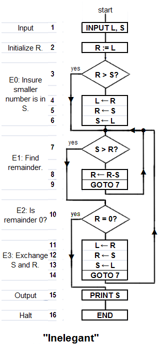
Wikimedia Foundation. 2010.