Reduction (complexity)

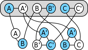Example of a reduction from a boolean satisfiability problem to a vertex cover problem. Blue vertices form a vertex cover which corresponds to truth values.

In computability theory and computational complexity theory, a reduction is a transformation of one problem into another problem. Depending on the transformation used this can be used to define complexity classes on a set of problems.

Intuitively, problem A is reducible to problem B if solutions to B exist and give solutions to A whenever A has solutions. Thus, solving A cannot be harder than solving B. We write A ≤_m B, usually with a subscript on the ≤ to indicate the type of reduction being used (m : mapping reduction, p : polynomial reduction).

Introduction

Often we find ourselves trying to solve a problem that is similar to a problem we've already solved. In these cases, often a quick way of solving the new problem is to transform each instance of the new problem into instances of the old problem, solve these using our existing solution, and then use these to obtain our final solution. This is perhaps the most obvious use of reductions.

Another, more subtle use is this: suppose we have a problem that we've proven is hard to solve, and we have a similar new problem. We might suspect that it, too, is hard to solve. We argue by contradiction: suppose the new problem is easy to solve. Then, if we can show that every instance of the old problem can be solved easily by transforming it into instances of the new problem and solving those, we have a contradiction. This establishes that the new problem is also hard.

A very simple example of a reduction is from multiplication to squaring. Suppose all we know how to do is to add, subtract, take squares, and divide by two. We can use this knowledge, combined with the following formula, to obtain the product of any two numbers:

$a \times b = \frac{\left(\left(a + b\right)^{2} - a^{2} - b^{2}\right)}{2}$

We also have a reduction in the other direction; obviously, if we can multiply two numbers, we can square a number. This seems to imply that these two problems are equally hard. This kind of reduction corresponds to Turing reduction.

However, the reduction becomes much harder if we add the restriction that we can only use the squaring function one time, and only at the end. In this case, even if we're allowed to use all the basic arithmetic operations, including multiplication, no reduction exists in general, because we may have to compute an irrational number like $\sqrt{2}$ from rational numbers. Going in the other direction, however, we can certainly square a number with just one multiplication, only at the end. Using this limited form of reduction, we have shown the unsurprising result that multiplication is harder in general than squaring. This corresponds to many-one reduction.

Definition

Given two subsets A and B of N and a set of functions F from N to N which is closed under composition, A is called reducible to B under F if

$\exists f \in F \mbox{ . } \forall x \in \mathbb{N} \mbox{ . } x \in A \Leftrightarrow f(x) \in B$

We write

$A \leq_{F} B$

Let S be a subset of P(N) and ≤ a reduction, then S is called closed under ≤ if

$\forall s \in S \mbox{ . } \forall A \in P(\mathbb{N}) \mbox{ . } A \leq s \Rightarrow A \in S$

A subset A of N is called hard for S if

$\forall s \in S \mbox{ . } s \leq A$

A subset A of N is called complete for S if A is hard for S and A is in S.

Properties

A reduction is a preordering, that is a reflexive and transitive relation, on P(N)×P(N), where P(N) is the power set of the natural numbers.

Types and applications of reductions

As described in the example above, there are two main types of reductions used in computational complexity, the many-one reduction and the Turing reduction. Many-one reductions map instances of one problem to instances of another; Turing reductions compute the solution to one problem, assuming the other problem is easy to solve. A many-one reduction is weaker than a Turing reduction. Weaker reductions are more effective at separating problems, but they have less power, making reductions harder to design.

A problem is complete for a complexity class if every problem in the class reduces to that problem, and it is also in the class itself. In this sense the problem represents the class, since any solution to it can, in combination with the reductions, be used to solve every problem in the class.

However, in order to be useful, reductions must be easy. For example, it's quite possible to reduce a difficult-to-solve NP-complete problem like the boolean satisfiability problem to a trivial problem, like determining if a number equals zero, by having the reduction machine solve the problem in exponential time and output zero only if there is a solution. However, this does not achieve much, because even though we can solve the new problem, performing the reduction is just as hard as solving the old problem. Likewise, a reduction computing a noncomputable function can reduce an undecidable problem to a decidable one. As Michael Sipser points out in Introduction to the Theory of Computation: "The reduction must be easy, relative to the complexity of typical problems in the class [...] If the reduction itself were difficult to compute, an easy solution to the complete problem wouldn't necessarily yield an easy solution to the problems reducing to it."

Therefore, the appropriate notion of reduction depends on the complexity class being studied. When studying the complexity class NP and harder classes such as the polynomial hierarchy, polynomial-time reductions are used. When studying classes within P such as NC and NL, log-space reductions are used. Reductions are also used in computability theory to show whether problems are or are not solvable by machines at all; in this case, reductions are restricted only to computable functions.

In case of optimization (maximization or minimization) problems, we often think in terms of approximation-preserving reductions. Suppose we have two optimization problems such that instances of one problem can be mapped onto instances of the other, in a way that nearly-optimal solutions to instances of the latter problem can be transformed back to yield nearly-optimal solutions to the former. This way, if we have an optimization algorithm (or approximation algorithm) that finds near-optimal (or optimal) solutions to instances of problem B, and an efficient approximation-preserving reduction from problem A to problem B, by composition we obtain an optimization algorithm that yields near-optimal solutions to instances of problem A. Approximation-preserving reductions are often used to prove hardness of approximation results: if some optimization problem A is hard to approximate (under some complexity assumption) within a factor better than α for some α, and there is a β-approximation-preserving reduction from problem A to problem B, we can conclude that problem B is hard to approximate within factor α/β.

Examples

• To show that a decision problem P is undecidable we must find a reduction from a decision problem which is already known to be undecidable to P. That reduction function must be a computable function. In particular, we often show that a problem P is undecidable by showing that the halting problem reduces to P.
• The complexity classes P, NP and PSPACE are closed under polynomial-time reductions.
• The complexity classes L, NL, P, NP and PSPACE are closed under log-space reduction.

Detailed example

The following example shows how to use reduction from the halting problem to prove that a language is undecidable. Suppose H(M, w) is the problem of determining whether a given Turing machine M halts (by accepting or rejecting) on input string w. This language is known to be undecidable. Suppose E(M) is the problem of determining whether the language a given Turing machine M accepts is empty (in other words, whether M accepts any strings at all). We show that E is undecidable by a reduction from H.

To obtain a contradiction, suppose R is a decider for E. We will use this to produce a decider S for H (which we know does not exist). Given input M and w (a Turing machine and some input string), define S(M, w) with the following behavior: S creates a Turing machine N that accepts only if the input string to N is w and M halts on input w, and does not halt otherwise. The decider S can now evaluate R(N) to check whether the language accepted by N is empty. If R accepts N, then the language accepted by N is empty, so in particular M does not halt on input w, so S can reject. If R rejects N, then the language accepted by N is nonempty, so M does halt on input w, so S can accept. Thus, if we had a decider R for E, we would be able to produce a decider S for the halting problem H(M, w) for any machine M and input w. Since we know that such an S cannot exist, it follows that the language E is also undecidable.

See also

• Reduction (recursion theory)
• Many-one reduction
• Truth table reduction
• Turing reduction
• Optimization (computer science)

External links

References

• Thomas H. Cormen, Charles E. Leiserson, Ronald L. Rivest and Clifford Stein, Introduction to Algorithms, MIT Press, 2001, ISBN 978-0-262-03293-3
• Hartley Rogers, Jr.: Theory of Recursive Functions and Effective Computability, McGraw-Hill, 1967, ISBN 978-0-262-68052-3.
• Peter Bürgisser: Completeness and Reduction in Algebraic Complexity Theory, Springer, 2000, ISBN 978-3-540-66752-0.
• E.R. Griffor: Handbook of Computability Theory, North Holland, 1999, ISBN 978-0-444-89882-1.