Turing machine

For the test of artificial intelligence, see Turing test. For the instrumental rock band, see Turing Machine (band).

Turing machine(s)
Machina
Universal Turing machine Alternating Turing machine Quantum Turing machine Read-only Turing machine Read-only right moving Turing Machines Probabilistic Turing machine Multi-track Turing machine Turing machine equivalents Turing machine examples Wolfram's 2-state 3-symbol..
Science
Alan Turing Category:Turing machine
This box: view · An artistic representation of a Turing machine (Rules table not represented) A Turing machine is a theoretical device that manipulates symbols on a strip of tape according to a table of rules. Despite its simplicity, a Turing machine can be adapted to simulate the logic of any computer algorithm, and is particularly useful in explaining the functions of a CPU inside a computer. The "Turing" machine was described by Alan Turing in 1936,[1] who called it an "a(utomatic)-machine". The Turing machine is not intended as a practical computing technology, but rather as a thought experiment representing a computing machine. Turing machines help computer scientists understand the limits of mechanical computation. Turing gave a succinct definition of the experiment in his 1948 essay, "Intelligent Machinery". Referring to his 1936 publication, Turing wrote that the Turing machine, here called a Logical Computing Machine, consisted of: ...an infinite memory capacity obtained in the form of an infinite tape marked out into squares, on each of which a symbol could be printed. At any moment there is one symbol in the machine; it is called the scanned symbol. The machine can alter the scanned symbol and its behavior is in part determined by that symbol, but the symbols on the tape elsewhere do not affect the behavior of the machine. However, the tape can be moved back and forth through the machine, this being one of the elementary operations of the machine. Any symbol on the tape may therefore eventually have an innings.[2] (Turing 1948, p. 61) A Turing machine that is able to simulate any other Turing machine is called a universal Turing machine (UTM, or simply a universal machine). A more mathematically-oriented definition with a similar "universal" nature was introduced by Alonzo Church, whose work on lambda calculus intertwined with Turing's in a formal theory of computation known as the Church–Turing thesis. The thesis states that Turing machines indeed capture the informal notion of effective method in logic and mathematics, and provide a precise definition of an algorithm or 'mechanical procedure'. Studying their abstract properties yields many insights into computer science and complexity theory.[3] Informal description For visualizations of Turing machines, see Turing machine gallery. The Turing machine mathematically models a machine that mechanically operates on a tape. On this tape are symbols which the machine can read and write, one at a time, using a tape head. Operation is fully determined by a finite set of elementary instructions such as "in state 42, if the symbol seen is 0, write a 1; if the symbol seen is 1, shift to the right, and change into state 17; in state 17, if the symbol seen is 0, write a 1 and change to state 6;" etc. In the original article ("On computable numbers, with an application to the Entscheidungsproblem", see also references below), Turing imagines not a mechanism, but a person whom he calls the "computer", who executes these deterministic mechanical rules slavishly (or as Turing puts it, "in a desultory manner"). The head is always over a particular square of the tape; only a finite stretch of squares is given. The instruction to be performed (q4) is shown over the scanned square. (Drawing after Kleene (1952) p.375.) 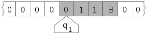Here, the internal state (q1) is shown inside the head, and the illustration describes the tape as being infinite and pre-filled with "0", the symbol serving as blank. The system's full state (its configuration) consists of the internal state, the contents of the shaded squares including the blank scanned by the head ("11B"), and the position of the head. (Drawing after Minsky (1967) p. 121). More precisely, a Turing machine consists of: A tape which is divided into cells, one next to the other. Each cell contains a symbol from some finite alphabet. The alphabet contains a special blank symbol (here written as 'B') and one or more other symbols. The tape is assumed to be arbitrarily extendable to the left and to the right, i.e., the Turing machine is always supplied with as much tape as it needs for its computation. Cells that have not been written to before are assumed to be filled with the blank symbol. In some models the tape has a left end marked with a special symbol; the tape extends or is indefinitely extensible to the right. A head that can read and write symbols on the tape and move the tape left and right one (and only one) cell at a time. In some models the head moves and the tape is stationary. A finite table (occasionally called an action table or transition function) of instructions (usually quintuples [5-tuples] : qiaj→qi1aj1dk, but sometimes 4-tuples) that, given the state(qi) the machine is currently in and the symbol(aj) it is reading on the tape (symbol currently under the head) tells the machine to do the following in sequence (for the 5-tuple models): Either erase or write a symbol (instead of aj, write aj1), and then Move the head (which is described by dk and can have values: 'L' for one step left or 'R' for one step right or 'N' for staying in the same place), and then Assume the same or a new state as prescribed (go to state qi1). In the 4-tuple models, erase or write a symbol (aj1) and move the head left or right (dk) are specified as separate instructions. Specifically, the table tells the machine to (ia) erase or write a symbol or (ib) move the head left or right, and then (ii) assume the same or a new state as prescribed, but not both actions (ia) and (ib) in the same instruction. In some models, if there is no entry in the table for the current combination of symbol and state then the machine will halt; other models require all entries to be filled. A state register that stores the state of the Turing machine, one of finitely many. There is one special start state with which the state register is initialized. These states, writes Turing, replace the "state of mind" a person performing computations would ordinarily be in. Note that every part of the machine—its state and symbol-collections—and its actions—printing, erasing and tape motion—is finite, discrete and distinguishable; it is the potentially unlimited amount of tape that gives it an unbounded amount of storage space. Examples of Turing machines To see examples of the following models, see Turing machine examples: Turing's very first machine Copy routine 3-state busy beaver Formal definition Hopcroft and Ullman (1979, p. 148) formally define a (one-tape) Turing machine as a 7-tuple $M= \langle Q, \Gamma, b, \Sigma, \delta, q_0, F \rangle$ where Q is a finite, non-empty set of states Γ is a finite, non-empty set of the tape alphabet/symbols $b \in \Gamma$ is the blank symbol (the only symbol allowed to occur on the tape infinitely often at any step during the computation) $\Sigma\subseteq\Gamma\setminus\{b\}$ is the set of input symbols $q_0 \in Q$ is the initial state $F \subseteq Q$ is the set of final or accepting states. $\delta: Q \setminus F \times \Gamma \rightarrow Q \times \Gamma \times \{L,R\}$ is a partial function called the transition function, where L is left shift, R is right shift. (A relatively uncommon variant allows "no shift", say N, as a third element of the latter set.) Anything that operates according to these specifications is a Turing machine. The 7-tuple for the 3-state busy beaver looks like this (see more about this busy beaver at Turing machine examples): Q = { A, B, C, HALT } Γ = { 0, 1 } b = 0 = "blank" Σ = { 1 } δ = see state-table below q0 = A = initial state F = the one element set of final states {HALT} Initially all tape cells are marked with 0. State table for 3 state, 2 symbol busy beaver Tape symbol Current state A Current state B Current state C Write symbol Move tape Next state Write symbol Move tape Next state Write symbol Move tape Next state 0 1 R B 1 L A 1 L B 1 1 L C 1 R B 1 R HALT Additional details required to visualize or implement Turing machines In the words of van Emde Boas (1990), p. 6: "The set-theoretical object [his formal seven-tuple description similar to the above] provides only partial information on how the machine will behave and what its computations will look like." For instance, There will need to be some decision on what the symbols actually look like, and a failproof way of reading and writing symbols indefinitely. The shift left and shift right operations may shift the tape head across the tape, but when actually building a Turing machine it is more practical to make the tape slide back and forth under the head instead. The tape can be finite, and automatically extended with blanks as needed (which is closest to the mathematical definition), but it is more common to think of it as stretching infinitely at both ends and being pre-filled with blanks except on the explicitly given finite fragment the tape head is on. (This is, of course, not implementable in practice.) The tape cannot be fixed in length, since that would not correspond to the given definition and would seriously limit the range of computations the machine can perform to those of a linear bounded automaton. Alternative definitions Definitions in literature sometimes differ slightly, to make arguments or proofs easier or clearer, but this is always done in such a way that the resulting machine has the same computational power. For example, changing the set {L,R} to {L,R,N}, where N ("None" or "No-operation") would allow the machine to stay on the same tape cell instead of moving left or right, does not increase the machine's computational power. The most common convention represents each "Turing instruction" in a "Turing table" by one of nine 5-tuples, per the convention of Turing/Davis (Turing (1936) in Undecidable, p. 126-127 and Davis (2000) p. 152): (definition 1): (qi, Sj, Sk/E/N, L/R/N, qm) ( current state qi , symbol scanned Sj , print symbol Sk/erase E/none N , move_tape_one_square left L/right R/none N , new state qm ) Other authors (Minsky (1967) p. 119, Hopcroft and Ullman (1979) p. 158, Stone (1972) p. 9) adopt a different convention, with new state qm listed immediately after the scanned symbol Sj: (definition 2): (qi, Sj, qm, Sk/E/N, L/R/N) ( current state qi , symbol scanned Sj , new state qm , print symbol Sk/erase E/none N , move_tape_one_square left L/right R/none N ) For the remainder of this article "definition 1" (the Turing/Davis convention) will be used. Example: state table for the 3-state 2-symbol busy beaver reduced to 5-tuples Current state Scanned symbol Print symbol Move tape Final (i.e. next) state 5-tuples A 0 1 R B (A, 0, 1, R, B) A 1 1 L C (A, 1, 1, L, C) B 0 1 L A (B, 0, 1, L, A) B 1 1 R B (B, 1, 1, R, B) C 0 1 L B (C, 0, 1, L, B) C 1 1 N H (C, 1, 1, N, H) In the following table, Turing's original model allowed only the first three lines that he called N1, N2, N3 (cf Turing in Undecidable, p. 126). He allowed for erasure of the "scanned square" by naming a 0th symbol S0 = "erase" or "blank", etc. However, he did not allow for non-printing, so every instruction-line includes "print symbol Sk" or "erase" (cf footnote 12 in Post (1947), Undecidable p. 300). The abbreviations are Turing's (Undecidable p. 119). Subsequent to Turing's original paper in 1936–1937, machine-models have allowed all nine possible types of five-tuples: Current m-configuration (Turing state) Tape symbol Print-operation Tape-motion Final m-configuration (Turing state) 5-tuple 5-tuple comments 4-tuple N1 qi Sj Print(Sk) Left L qm (qi, Sj, Sk, L, qm) "blank" = S0, 1=S1, etc. N2 qi Sj Print(Sk) Right R qm (qi, Sj, Sk, R, qm) "blank" = S0, 1=S1, etc. N3 qi Sj Print(Sk) None N qm (qi, Sj, Sk, N, qm) "blank" = S0, 1=S1, etc. (qi, Sj, Sk, qm) 4 qi Sj None N Left L qm (qi, Sj, N, L, qm) (qi, Sj, L, qm) 5 qi Sj None N Right R qm (qi, Sj, N, R, qm) (qi, Sj, R, qm) 6 qi Sj None N None N qm (qi, Sj, N, N, qm) Direct "jump" (qi, Sj, N, qm) 7 qi Sj Erase Left L qm (qi, Sj, E, L, qm) 8 qi Sj Erase Right R qm (qi, Sj, E, R, qm) 9 qi Sj Erase None N qm (qi, Sj, E, N, qm) (qi, Sj, E, qm) Any Turing table (list of instructions) can be constructed from the above nine 5-tuples. For technical reasons, the three non-printing or "N" instructions (4, 5, 6) can usually be dispensed with. For examples see Turing machine examples. Less frequently the use of 4-tuples are encountered: these represent a further atomization of the Turing instructions (cf Post (1947), Boolos & Jeffrey (1974, 1999), Davis-Sigal-Weyuker (1994)); also see more at Post–Turing machine. The "state" The word "state" used in context of Turing machines can be a source of confusion, as it can mean two things. Most commentators after Turing have used "state" to mean the name/designator of the current instruction to be performed—i.e. the contents of the state register. But Turing (1936) made a strong distinction between a record of what he called the machine's "m-configuration", (its internal state) and the machine's (or person's) "state of progress" through the computation - the current state of the total system. What Turing called "the state formula" includes both the current instruction and all the symbols on the tape: Thus the state of progress of the computation at any stage is completely determined by the note of instructions and the symbols on the tape. That is, the state of the system may be described by a single expression (sequence of symbols) consisting of the symbols on the tape followed by Δ (which we suppose not to appear elsewhere) and then by the note of instructions. This expression is called the 'state formula'. —Undecidable, p.139–140, emphasis added Earlier in his paper Turing carried this even further: he gives an example where he places a symbol of the current "m-configuration"—the instruction's label—beneath the scanned square, together with all the symbols on the tape (Undecidable, p. 121); this he calls "the complete configuration" (Undecidable, p. 118). To print the "complete configuration" on one line he places the state-label/m-configuration to the left of the scanned symbol. A variant of this is seen in Kleene (1952) where Kleene shows how to write the Gödel number of a machine's "situation": he places the "m-configuration" symbol q4 over the scanned square in roughly the center of the 6 non-blank squares on the tape (see the Turing-tape figure in this article) and puts it to the right of the scanned square. But Kleene refers to "q4" itself as "the machine state" (Kleene, p. 374-375). Hopcroft and Ullman call this composite the "instantaneous description" and follow the Turing convention of putting the "current state" (instruction-label, m-configuration) to the left of the scanned symbol (p. 149). Example: total state of 3-state 2-symbol busy beaver after 3 "moves" (taken from example "run" in the figure below): 1A1 This means: after three moves the tape has ... 000110000 ... on it, the head is scanning the right-most 1, and the state is A. Blanks (in this case represented by "0"s) can be part of the total state as shown here: B01 ; the tape has a single 1 on it, but the head is scanning the 0 ("blank") to its left and the state is B. "State" in the context of Turing machines should be clarified as to which is being described: (i) the current instruction, or (ii) the list of symbols on the tape together with the current instruction, or (iii) the list of symbols on the tape together with the current instruction placed to the left of the scanned symbol or to the right of the scanned symbol. Turing's biographer Andrew Hodges (1983: 107) has noted and discussed this confusion. 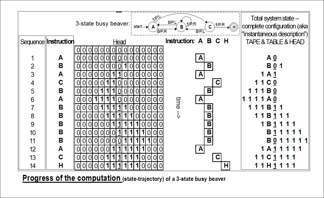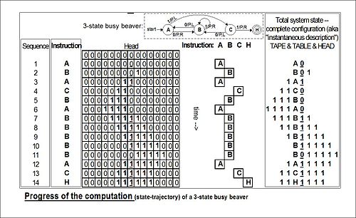Turing machine "state" diagrams The table for the 3-state busy beaver ("P" = print/write a "1") Tape symbol Current state A Current state B Current state C Write symbol Move tape Next state Write symbol Move tape Next state Write symbol Move tape Next state 0 P R B P L A P L B 1 P L C P R B P R HALT 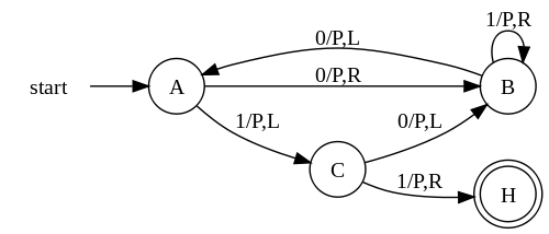The "3-state busy beaver" Turing Machine in a finite state representation. Each circle represents a "state" of the TABLE—an "m-configuration" or "instruction". "Direction" of a state transition is shown by an arrow. The label (e.g.. 0/P,R) near the outgoing state (at the "tail" of the arrow) specifies the scanned symbol that causes a particular transition (e.g. 0) followed by a slash /, followed by the subsequent "behaviors" of the machine, e.g. "P Print" then move tape "R Right". No general accepted format exists. The convention shown is after McClusky (1965), Booth (1967), Hill and Peterson (1974). To the right: the above TABLE as expressed as a "state transition" diagram. Usually large TABLES are better left as tables (Booth, p. 74). They are more readily simulated by computer in tabular form (Booth, p. 74). However, certain concepts—e.g. machines with "reset" states and machines with repeating patterns (cf Hill and Peterson p. 244ff)—can be more readily seen when viewed as a drawing. Whether a drawing represents an improvement on its TABLE must be decided by the reader for the particular context. See Finite state machine for more. The evolution of the busy-beaver's computation starts at the top and proceeds to the bottom. The reader should again be cautioned that such diagrams represent a snapshot of their TABLE frozen in time, not the course ("trajectory") of a computation through time and/or space. While every time the busy beaver machine "runs" it will always follow the same state-trajectory, this is not true for the "copy" machine that can be provided with variable input "parameters". The diagram "Progress of the computation" shows the 3-state busy beaver's "state" (instruction) progress through its computation from start to finish. On the far right is the Turing "complete configuration" (Kleene "situation", Hopcroft–Ullman "instantaneous description") at each step. If the machine were to be stopped and cleared to blank both the "state register" and entire tape, these "configurations" could be used to rekindle a computation anywhere in its progress (cf Turing (1936) Undecidable pp. 139–140). Models equivalent to the Turing machine model See also: Turing machine equivalents, Register machine, and Post–Turing machine Many machines that might be thought to have more computational capability than a simple universal Turing machine can be shown to have no more power (Hopcroft and Ullman p. 159, cf Minsky (1967)). They might compute faster, perhaps, or use less memory, or their instruction set might be smaller, but they cannot compute more powerfully (i.e. more mathematical functions). (Recall that the Church–Turing thesis hypothesizes this to be true for any kind of machine: that anything that can be "computed" can be computed by some Turing machine.) A Turing machine is equivalent to a pushdown automaton that has been made more flexible and concise by relaxing the last-in-first-out requirement of its stack. At the other extreme, some very simple models turn out to be Turing-equivalent, i.e. to have the same computational power as the Turing machine model. Common equivalent models are the multi-tape Turing machine, multi-track Turing machine, machines with input and output, and the non-deterministic Turing machine (NDTM) as opposed to the deterministic Turing machine (DTM) for which the action table has at most one entry for each combination of symbol and state. Read-only, right-moving Turing Machines are equivalent to NDFA's (as well as DFA's by conversion using the NDFA to DFA conversion algorithm). For practical and didactical intentions the equivalent register machine can be used as a usual assembly programming language. Choice c-machines, Oracle o-machines Early in his paper (1936) Turing makes a distinction between an "automatic machine"—its "motion ... completely determined by the configuration" and a "choice machine": ...whose motion is only partially determined by the configuration ... When such a machine reaches one of these ambiguous configurations, it cannot go on until some arbitrary choice has been made by an external operator. This would be the case if we were using machines to deal with axiomatic systems. —Undecidable, p. 118 Turing (1936) does not elaborate further except in a footnote in which he describes how to use an a-machine to "find all the provable formulae of the [Hilbert] calculus" rather than use a choice machine. He "suppose[s] that the choices are always between two possibilities 0 and 1. Each proof will then be determined by a sequence of choices i1, i2, ..., in (i1 = 0 or 1, i2 = 0 or 1, ..., in = 0 or 1), and hence the number 2n + i12n-1 + i22n-2 + ... +in completely determines the proof. The automatic machine carries out successively proof 1, proof 2, proof 3, ..." (Footnote ‡, Undecidable, p. 138) This is indeed the technique by which a deterministic (i.e. a-) Turing machine can be used to mimic the action of a nondeterministic Turing machine; Turing solved the matter in a footnote and appears to dismiss it from further consideration. An oracle machine or o-machine is a Turing a-machine that pauses its computation at state "o" while, to complete its calculation, it "awaits the decision" of "the oracle"—an unspecified entity "apart from saying that it cannot be a machine" (Turing (1939), Undecidable p. 166–168). The concept is now actively used by mathematicians. Universal Turing machines Main article: Universal Turing machine As Turing wrote in Undecidable, p. 128 (italics added): It is possible to invent a single machine which can be used to compute any computable sequence. If this machine U is supplied with the tape on the beginning of which is written the string of quintuples separated by semicolons of some computing machine M, then U will compute the same sequence as M. This finding is now taken for granted, but at the time (1936) it was considered astonishing. The model of computation that Turing called his "universal machine"—"U" for short—is considered by some (cf Davis (2000)) to have been the fundamental theoretical breakthrough that led to the notion of the Stored-program computer. Turing's paper ... contains, in essence, the invention of the modern computer and some of the programming techniques that accompanied it. —Minsky (1967), p. 104 In terms of computational complexity, a multi-tape universal Turing machine need only be slower by logarithmic factor compared to the machines it simulates. This result was obtained in 1966 by F. C. Hennie and R. E. Stearns. (Arora and Barak, 2009, theorem 1.9) Comparison with real machines It is often said that Turing machines, unlike simpler automata, are as powerful as real machines, and are able to execute any operation that a real program can. What is missed in this statement is that, because a real machine can only be in finitely many configurations, in fact this "real machine" is nothing but a linear bounded automaton. On the other hand, Turing machines are equivalent to machines that have an unlimited amount of storage space for their computations. In fact, Turing machines are not intended to model computers, but rather they are intended to model computation itself; historically, computers, which compute only on their (fixed) internal storage, were developed only later. There are a number of ways to explain why Turing machines are useful models of real computers: Anything a real computer can compute, a Turing machine can also compute. For example: "A Turing machine can simulate any type of subroutine found in programming languages, including recursive procedures and any of the known parameter-passing mechanisms" (Hopcroft and Ullman p. 157). A large enough FSA can also model any real computer, disregarding IO. Thus, a statement about the limitations of Turing machines will also apply to real computers. The difference lies only with the ability of a Turing machine to manipulate an unbounded amount of data. However, given a finite amount of time, a Turing machine (like a real machine) can only manipulate a finite amount of data. Like a Turing machine, a real machine can have its storage space enlarged as needed, by acquiring more disks or other storage media. If the supply of these runs short, the Turing machine may become less useful as a model. But the fact is that neither Turing machines nor real machines need astronomical amounts of storage space in order to perform useful computation. The processing time required is usually much more of a problem. Descriptions of real machine programs using simpler abstract models are often much more complex than descriptions using Turing machines. For example, a Turing machine describing an algorithm may have a few hundred states, while the equivalent deterministic finite automaton on a given real machine has quadrillions. This makes the DFA representation infeasible to analyze. Turing machines describe algorithms independent of how much memory they use. There is a limit to the memory possessed by any current machine, but this limit can rise arbitrarily in time. Turing machines allow us to make statements about algorithms which will (theoretically) hold forever, regardless of advances in conventional computing machine architecture. Turing machines simplify the statement of algorithms. Algorithms running on Turing-equivalent abstract machines are usually more general than their counterparts running on real machines, because they have arbitrary-precision data types available and never have to deal with unexpected conditions (including, but not limited to, running out of memory). One way in which Turing machines are a poor model for programs is that many real programs, such as operating systems and word processors, are written to receive unbounded input over time, and therefore do not halt. Turing machines do not model such ongoing computation well (but can still model portions of it, such as individual procedures). Limitations of Turing machines Computational Complexity Theory Further information: Computational complexity theory A limitation of Turing Machines is that they do not model the strengths of a particular arrangement well. For instance, modern stored-program computers are actually instances of a more specific form of abstract machine known as the random access stored program machine or RASP machine model. Like the Universal Turing machine the RASP stores its "program" in "memory" external to its finite-state machine's "instructions". Unlike the Universal Turing Machine, the RASP has an infinite number of distinguishable, numbered but unbounded "registers"—memory "cells" that can contain any integer (cf. Elgot and Robinson (1964), Hartmanis (1971), and in particular Cook-Rechow (1973); references at random access machine). The RASP's finite-state machine is equipped with the capability for indirect addressing (e.g. the contents of one register can be used as an address to specify another register); thus the RASP's "program" can address any register in the register-sequence. The upshot of this distinction is that there are computational optimizations that can be performed based on the memory indices, which are not possible in a general Turing Machine; thus when Turing Machines are used as the basis for bounding running times, a 'false lower bound' can be proven on certain algorithms' running times (due to the false simplifying assumption of a Turing Machine). An example of this is binary search, an algorithm that can be shown to perform more quickly when using the RASP model of computation rather than the Turing machine model. Concurrency Another limitation of Turing machines is that they do not model concurrency well. For example, there is a bound on the size of integer that can be computed by an always-halting nondeterministic Turing Machine starting on a blank tape. (See article on Unbounded nondeterminism.) By contrast, there are always-halting concurrent systems with no inputs that can compute an integer of unbounded size. (A process can be created with local storage that is initialized with a count of 0 that concurrently sends itself both a stop and a go message. When it receives a go message, it increments its count by 1 and sends itself a go message. When it receives a stop message, it stops with an unbounded number in its local storage.) History See also: Algorithm and Church–Turing thesis They were described in 1936 by Alan Turing. Historical background: computational machinery Robin Gandy (1919–1995)—a student of Alan Turing (1912–1954) and his life-long friend—traces the lineage of the notion of "calculating machine" back to Babbage (circa 1834) and actually proposes "Babbage's Thesis": That the whole of development and operations of analysis are now capable of being executed by machinery. —(italics in Babbage as cited by Gandy, p. 54) Gandy's analysis of Babbage's Analytical Engine describes the following five operations (cf p. 52–53): The arithmetic functions +, −, × where − indicates "proper" subtraction x − y = 0 if y ≥ x Any sequence of operations is an operation Iteration of an operation (repeating n times an operation P) Conditional iteration (repeating n times an operation P conditional on the "success" of test T) Conditional transfer (i.e. conditional "goto") Gandy states that "the functions which can be calculated by (1), (2), and (4) are precisely those which are Turing computable." (p. 53). He cites other proposals for "universal calculating machines" included those of Percy Ludgate (1909), Leonardo Torres y Quevedo (1914), Maurice d'Ocagne (1922), Louis Couffignal (1933), Vannevar Bush (1936), Howard Aiken (1937). However: ... the emphasis is on programming a fixed iterable sequence of arithmetical operations. The fundamental importance of conditional iteration and conditional transfer for a general theory of calculating machines is not recognized ... —Gandy p. 55 The Entscheidungsproblem (the "decision problem"): Hilbert's tenth question of 1900 With regards to Hilbert's problems posed by the famous mathematician David Hilbert in 1900, an aspect of problem #10 had been floating about for almost 30 years before it was framed precisely. Hilbert's original expression for #10 is as follows: 10. Determination of the solvability of a Diophantine equation. Given a Diophantine equation with any number of unknown quantities and with rational integral coefficients: To devise a process according to which it can be determined in a finite number of operations whether the equation is solvable in rational integers. The Entscheidungsproblem [decision problem for first-order logic] is solved when we know a procedure that allows for any given logical expression to decide by finitely many operations its validity or satisfiability ... The Entscheidungsproblem must be considered the main problem of mathematical logic. —quoted, with this translation and the original German, in Dershowitz and Gurevich, 2008 By 1922, this notion of "Entscheidungsproblem" had developed a bit, and H. Behmann stated that ... most general form of the Entscheidungsproblem [is] as follows: A quite definite generally applicable prescription is required which will allow one to decide in a finite number of steps the truth or falsity of a given purely logical assertion ... —Gandy p. 57, quoting Behmann Behmann remarks that ... the general problem is equivalent to the problem of deciding which mathematical propositions are true. —ibid. If one were able to solve the Entscheidungsproblem then one would have a "procedure for solving many (or even all) mathematical problems". —ibid., p. 92 By the 1928 international congress of mathematicians Hilbert "made his questions quite precise. First, was mathematics complete ... Second, was mathematics consistent ... And thirdly, was mathematics decidable?" (Hodges p. 91, Hawking p. 1121). The first two questions were answered in 1930 by Kurt Gödel at the very same meeting where Hilbert delivered his retirement speech (much to the chagrin of Hilbert); the third—the Entscheidungsproblem—had to wait until the mid-1930s. The problem was that an answer first required a precise definition of "definite general applicable prescription", which Princeton professor Alonzo Church would come to call "effective calculability", and in 1928 no such definition existed. But over the next 6–7 years Emil Post developed his definition of a worker moving from room to room writing and erasing marks per a list of instructions (Post 1936), as did Church and his two students Stephen Kleene and J. B. Rosser by use of Church's lambda-calculus and Gödel's recursion theory (1934). Church's paper (published 15 April 1936) showed that the Entscheidungsproblem was indeed "undecidable" and beat Turing to the punch by almost a year (Turing's paper submitted 28 May 1936, published January 1937). In the meantime, Emil Post submitted a brief paper in the fall of 1936, so Turing at least had priority over Post. While Church refereed Turing's paper, Turing had time to study Church's paper and add an Appendix where he sketched a proof that Church's lambda-calculus and his machines would compute the same functions. But what Church had done was something rather different, and in a certain sense weaker. ... the Turing construction was more direct, and provided an argument from first principles, closing the gap in Church's demonstration. —Hodges p. 112 And Post had only proposed a definition of calculability and criticized Church's "definition", but had proved nothing. Alan Turing's a- (automatic-)machine In the spring of 1935 Turing as a young Master's student at King's College Cambridge, UK, took on the challenge; he had been stimulated by the lectures of the logician M. H. A. Newman "and learned from them of Gödel's work and the Entscheidungsproblem ... Newman used the word 'mechanical' ... In his obituary of Turing 1955 Newman writes: To the question 'what is a "mechanical" process?' Turing returned the characteristic answer 'Something that can be done by a machine' and he embarked on the highly congenial task of analysing the general notion of a computing machine. —Gandy, p. 74 Gandy states that: I suppose, but do not know, that Turing, right from the start of his work, had as his goal a proof of the undecidability of the Entscheidungsproblem. He told me that the 'main idea' of the paper came to him when he was lying in Grantchester meadows in the summer of 1935. The 'main idea' might have either been his analysis of computation or his realization that there was a universal machine, and so a diagonal argument to prove unsolvability. —ibid., p. 76 While Gandy believed that Newman's statement above is "misleading", this opinion is not shared by all. Turing had a life-long interest in machines: "Alan had dreamt of inventing typewriters as a boy; [his mother] Mrs. Turing had a typewriter; and he could well have begun by asking himself what was meant by calling a typewriter 'mechanical'" (Hodges p. 96). While at Princeton pursuing his PhD, Turing built a Boolean-logic multiplier (see below). His PhD thesis, titled "Systems of Logic Based on Ordinals", contains the following definition of "a computable function": It was stated above that 'a function is effectively calculable if its values can be found by some purely mechanical process'. We may take this statement literally, understanding by a purely mechanical process one which could be carried out by a machine. It is possible to give a mathematical description, in a certain normal form, of the structures of these machines. The development of these ideas leads to the author's definition of a computable function, and to an identification of computability with effective calculability. It is not difficult, though somewhat laborious, to prove that these three definitions [the 3rd is the λ-calculus] are equivalent. —Turing (1939) in The Undecidable, p. 160 When Turing returned to the UK he ultimately became jointly responsible for breaking the German secret codes created by encryption machines called "The Enigma"; he also became involved in the design of the ACE (Automatic Computing Engine), "[Turing's] ACE proposal was effectively self-contained, and its roots lay not in the EDVAC [the USA's initiative], but in his own universal machine" (Hodges p. 318). Arguments still continue concerning the origin and nature of what has been named by Kleene (1952) Turing's Thesis. But what Turing did prove with his computational-machine model appears in his paper On Computable Numbers, With an Application to the Entscheidungsproblem (1937): [that] the Hilbert Entscheidungsproblem can have no solution ... I propose, therefore to show that there can be no general process for determining whether a given formula U of the functional calculus K is provable, i.e. that there can be no machine which, supplied with any one U of these formulae, will eventually say whether U is provable. —from Turing's paper as reprinted in The Undecidable, p. 145 Turing's example (his second proof): If one is to ask for a general procedure to tell us: "Does this machine ever print 0", the question is "undecidable". 1937–1970: The "digital computer", the birth of "computer science" In 1937, while at Princeton working on his PhD thesis, Turing built a digital (Boolean-logic) multiplier from scratch, making his own electromechanical relays (Hodges p. 138). "Alan's task was to embody the logical design of a Turing machine in a network of relay-operated switches ..." (Hodges p. 138). While Turing might have been just curious and experimenting, quite-earnest work in the same direction was going in Germany (Konrad Zuse (1938)), and in the United States (Howard Aiken) and George Stibitz (1937); the fruits of their labors were used by the Axis and Allied military in World War II (cf Hodges p. 298–299). In the early to mid-1950s Hao Wang and Marvin Minsky reduced the Turing machine to a simpler form (a precursor to the Post-Turing machine of Martin Davis); simultaneously European researchers were reducing the new-fangled electronic computer to a computer-like theoretical object equivalent to what was now being called a "Turing machine". In the late 1950s and early 1960s, the coincidentally-parallel developments of Melzak and Lambek (1961), Minsky (1961), and Shepherdson and Sturgis (1961) carried the European work further and reduced the Turing machine to a more friendly, computer-like abstract model called the counter machine; Elgot and Robinson (1964), Hartmanis (1971), Cook and Reckhow (1973) carried this work even further with the register machine and random access machine models—but basically all are just multi-tape Turing machines with an arithmetic-like instruction set. 1970–present: the Turing machine as a model of computation Today the counter, register and random-access machines and their sire the Turing machine continue to be the models of choice for theorists investigating questions in the theory of computation. In particular, computational complexity theory makes use of the Turing machine: Depending on the objects one likes to manipulate in the computations (numbers like nonnegative integers or alphanumeric strings), two models have obtained a dominant position in machine-based complexity theory: the off-line multitape Turing machine..., which represents the standard model for string-oriented computation, and the random access machine (RAM) as introduced by Cook and Reckhow ..., which models the idealized Von Neumann style computer. —van Emde Boas 1990:4 Only in the related area of analysis of algorithms this role is taken over by the RAM model. —van Emde Boas 1990:16 Kantorovitz (2005),[4] was the first to show the most simple obvious representation of Turing Machines published academically which unifies Turing Machines with mathematical analysis and analog computers. See also Algorithm, for a brief history of some of the inventions and the mathematics leading to Turing's definition of what he called his "a-machine" Arithmetical hierarchy Bekenstein bound; Because they have an infinite tape, Turing machines are physically impossible if they are to have a finite size and bounded energy. BlooP and FlooP Busy beaver Chaitin constant or Omega (computer science) for information relating to the halting problem Church-Turing thesis, which says Turing machines can perform any computation that can be performed Conway's Game of Life, a Turing-complete cellular automaton Genetix a virtual machine created by Bernard Hodson containing only 34 executable instructions. Gödel, Escher, Bach: An Eternal Golden Braid, an influential book largely about the Church-Turing Thesis. Halting problem, for more references Harvard architecture Hyperbrain a theoretical model of the brain Langton's ant and Turmites, simple two-dimensional analogues of the Turing machine. Modified Harvard architecture Probabilistic Turing machine Quantum Turing machine Turing completeness, an attribute used in computability theory to describe computing systems with power equivalent to a universal Turing machine. Turing switch Turing tarpit, any computing system or language which, despite being Turing complete, is generally considered useless for practical computing. Von Neumann architecture Notes ^ The idea came to him in mid-1935 (perhaps, see more in the History section) after a question posed by M. H. A. Newman in his lectures -- "Was there a definite method, or as Newman put it, a mechanical process which could be applied to a mathematical statement, and which would come up with the answer as to whether it was provable" (Hodges 1983:93). Turing submitted his paper on 31 May 1936 to the London Mathematical Society for its Proceedings (cf Hodges 1983:112), but it was published in early 1937 -- offprints available February 1937 (cf Hodges 1983:129). ^ See the definition of "innings" on Wiktionary ^ Vitanyi, Paul M.B. (2009). "Turing machine". Scholarpedia 4 (3): 6240. doi:10.4249/scholarpedia.6240. ISSN 1941-6016. http://www.scholarpedia.org/article/Turing_machine#Importance_of_the_Turing_machine. Retrieved 23 April 2010. "In the last three-quarter of a century the Turing machine model has proven to be of priceless value for the development of the science of dataprocessing. All theory development reaches back to this format. The model has become so dominant that new other models that are not polynomial-time reducible to Turing machines are viewed as not realistic (the so-called polynomial-time Computability thesis)."  ^ ACM.org; Isaiah Pinchas Kantorovitz (2005) - A note on turing machine computability of rule driven systems References Primary literature, reprints, and compilations B. Jack Copeland ed. (2004), The Essential Turing: Seminal Writings in Computing, Logic, Philosophy, Artificial Intelligence, and Artificial Life plus The Secrets of Enigma, Clarendon Press (Oxford University Press), Oxford UK, ISBN 0-19-825079-7. Contains the Turing papers plus a draft letter to Emil Post re his criticism of "Turing's convention", and Donald W. Davies' Corrections to Turing's Universal Computing Machine Martin Davis (ed.) (1965), The Undecidable, Raven Press, Hewlett, NY. Emil Post (1936), "Finite Combinatory Processes—Formulation 1", Journal of Symbolic Logic, 1, 103–105, 1936. Reprinted in The Undecidable pp. 289ff. Emil Post (1947), "Recursive Unsolvability of a Problem of Thue", Journal of Symbolic Logic, vol. 12, pp. 1–11. Reprinted in The Undecidable pp. 293ff. In the Appendix of this paper Post comments on and gives corrections to Turing's paper of 1936–1937. In particular see the footnotes 11 with corrections to the universal computing machine coding and footnote 14 with comments on Turing's first and second proofs. Turing, A.M. (1936). "On Computable Numbers, with an Application to the Entscheidungsproblem". Proceedings of the London Mathematical Society. 2 42: 230–65. 1937. doi:10.1112/plms/s2-42.1.230.  (and Turing, A.M. (1938). "On Computable Numbers, with an Application to the Entscheidungsproblem: A correction". Proceedings of the London Mathematical Society. 2 43 (6): 544–6. 1937. doi:10.1112/plms/s2-43.6.544. ). Reprinted in many collections, e.g. in The Undecidable pp. 115–154; available on the web in many places, e.g. at Scribd. Alan Turing, 1948, "Intelligent Machinery." Reprinted in "Cybernetics: Key Papers." Ed. C.R. Evans and A.D.J. Robertson. Baltimore: University Park Press, 1968. p. 31. F. C. Hennie and R. E. Stearns. Two-tape simulation of multitape Turing machines. JACM, 13(4):533–546, 1966. Computability theory Boolos, George; Richard Jeffrey (1989, 1999). Computability and Logic (3rd ed.). Cambridge UK: Cambridge University Press. ISBN 0-521-20402-X.  Boolos, George; John Burgess, Richard Jeffrey, (2002). Computability and Logic (4th ed.). Cambridge UK: Cambridge University Press. ISBN 0-521-00758-5 (pb.).  Some parts have been significantly rewritten by Burgess. Presentation of Turing machines in context of Lambek "abacus machines" (cf Register machine) and recursive functions, showing their equivalence. Taylor L. Booth (1967), Sequential Machines and Automata Theory, John Wiley and Sons, Inc., New York. Graduate level engineering text; ranges over a wide variety of topics, Chapter IX Turing Machines includes some recursion theory. Martin Davis (1958). Computability and Unsolvability. McGraw-Hill Book Company, Inc, New York. . On pages 12–20 he gives examples of 5-tuple tables for Addition, The Successor Function, Subtraction (x ≥ y), Proper Subtraction (0 if x < y), The Identity Function and various identity functions, and Multiplication. Davis, Martin; Ron Sigal, Elaine J. Weyuker (1994). Computability, Complexity, and Languages and Logic: Fundamentals of Theoretical Computer Science (2nd ed.). San Diego: Academic Press, Harcourt, Brace & Company. ISBN 0122063821.  Hennie, Fredrick (1977). Introduction to Computability. Addison–Wesley, Reading, Mass. . On pages 90–103 Hennie discusses the UTM with examples and flow-charts, but no actual 'code'. John Hopcroft and Jeffrey Ullman, (1979). Introduction to Automata Theory, Languages and Computation (1st ed.). Addison–Wesley, Reading Mass. ISBN 0-201-02988-X..  A difficult book. Centered around the issues of machine-interpretation of "languages", NP-completeness, etc. Hopcroft, John E.; Rajeev Motwani, Jeffrey D. Ullman (2001). Introduction to Automata Theory, Languages, and Computation (2nd ed.). Reading Mass: Addison–Wesley. ISBN 0201441241.  Distinctly different and less intimidating than the first edition. Stephen Kleene (1952), Introduction to Metamathematics, North–Holland Publishing Company, Amsterdam Netherlands, 10th impression (with corrections of 6th reprint 1971). Graduate level text; most of Chapter XIII Computable functions is on Turing machine proofs of computability of recursive functions, etc. Knuth, Donald E. (1973). Volume 1/Fundamental Algorithms: The Art of computer Programming (2nd ed.). Reading, Mass.: Addison–Wesley Publishing Company. . With reference to the role of Turing machines in the development of computation (both hardware and software) see 1.4.5 History and Bibliography pp. 225ff and 2.6 History and Bibliographypp. 456ff. Zohar Manna, 1974, Mathematical Theory of Computation. Reprinted, Dover, 2003. ISBN 9780486432380 Marvin Minsky, Computation: Finite and Infinite Machines, Prentice–Hall, Inc., N.J., 1967. See Chapter 8, Section 8.2 "Unsolvability of the Halting Problem." Excellent, i.e. relatively readable, sometimes funny. Christos Papadimitriou (1993). Computational Complexity (1st ed.). Addison Wesley. ISBN 0-201-53082-1.  Chapter 2: Turing machines, pp. 19–56. Michael Sipser (1997). Introduction to the Theory of Computation. PWS Publishing. ISBN 0-534-94728-X.  Chapter 3: The Church–Turing Thesis, pp. 125–149. Stone, Harold S. (1972). Introduction to Computer Organization and Data Structures (1st ed.). New York: McGraw–Hill Book Company. ISBN 0-07-061726-0.  Peter van Emde Boas 1990, Machine Models and Simulations, pp. 3–66, in Jan van Leeuwen, ed., Handbook of Theoretical Computer Science, Volume A: Algorithms and Complexity, The MIT Press/Elsevier, [place?], ISBN 0-444-88071-2 (Volume A). QA76.H279 1990. Valuable survey, with 141 references. Church's thesis Nachum Dershowitz; Yuri Gurevich (September 2008). "A natural axiomatization of computability and proof of Church's Thesis". Bulletin of Symbolic Logic 14 (3). http://research.microsoft.com/en-us/um/people/gurevich/Opera/188.pdf. Retrieved 2008-10-15.  Roger Penrose (1989, 1990). The Emperor's New Mind (2nd ed.). Oxford University Press, New York. ISBN 0-19-851973-7.  Small Turing machines Rogozhin, Yurii, 1998, "A Universal Turing Machine with 22 States and 2 Symbols", Romanian Journal Of Information Science and Technology, 1(3), 259–265, 1998. (surveys known results about small universal Turing machines) Stephen Wolfram, 2002, A New Kind of Science, Wolfram Media, ISBN 1-57955-008-8 Brunfiel, Geoff, Student snags maths prize, Nature, October 24. 2007. Jim Giles (2007), Simplest 'universal computer' wins student $25,000, New Scientist, October 24, 2007. Alex Smith, Universality of Wolfram’s 2, 3 Turing Machine, Submission for the Wolfram 2, 3 Turing Machine Research Prize. Vaughan Pratt, 2007, "Simple Turing machines, Universality, Encodings, etc.", FOM email list. October 29, 2007. Martin Davis, 2007, "Smallest universal machine", and Definition of universal Turing machine FOM email list. October 26–27, 2007. Alasdair Urquhart, 2007 "Smallest universal machine", FOM email list. October 26, 2007. Hector Zenil (Wolfram Research), 2007 "smallest universal machine", FOM email list. October 29, 2007. Todd Rowland, 2007, "Confusion on FOM", Wolfram Science message board, October 30, 2007. Other Martin Davis (2000). Engines of Logic: Mathematicians and the origin of the Computer (1st ed.). W. W. Norton & Company, New York. ISBN 0-393-32229-7 pbk..  Robin Gandy, "The Confluence of Ideas in 1936", pp. 51–102 in Rolf Herken, see below. Stephen Hawking (editor), 2005, God Created the Integers: The Mathematical Breakthroughs that Changed History, Running Press, Philadelphia, ISBN 978-0-7624-1922-7. Includes Turing's 1936–1937 paper, with brief commentary and biography of Turing as written by Hawking. Rolf Herken (1995). The Universal Turing Machine—A Half-Century Survey. Springer Verlag. ISBN 3-211-82637-8.  Andrew Hodges, Alan Turing: The Enigma, Simon and Schuster, New York. Cf Chapter "The Spirit of Truth" for a history leading to, and a discussion of, his proof. Ivars Peterson (1988). The Mathematical Tourist: Snapshots of Modern Mathematics (1st ed.). W. H. Freeman and Company, New York. ISBN 0-7167-2064-7 (pbk.).  Paul Strathern (1997). Turing and the Computer—The Big Idea. Anchor Books/Doubleday. ISBN 0-385-49243-X.  Hao Wang, "A variant to Turing's theory of computing machines", Journal of the Association for Computing Machinery (JACM) 4, 63–92 (1957). Charles Petzold, Petzold, Charles, The Annotated Turing, John Wiley & Sons, Inc., ISBN 0-47022-905-5 Arora, Sanjeev; Barak, Boaz, "Complexity Theory: A Modern Approach", Cambridge University Press, 2009, ISBN 978-0-521-42426-4, section 1.4, "Machines as strings and the universal Turing machine" and 1.7, "Proof of theorem 1.9" Isaiah Pinchas Kantorovitz, "A note on turing machine computability of rule driven systems", ACM SIGACT News December 2005. External links Turing Machine on Stanford Encyclopedia of Philosophy Detailed info on the Church–Turing Hypothesis (Stanford Encyclopedia of Philosophy) Turing Machine-Like Models in Molecular Biology, to understand life mechanisms with a DNA-tape processor. The Turing machine—Summary about the Turing machine, its functionality and historical facts The Wolfram 2,3 Turing Machine Research Prize—Stephen Wolfram's $25,000 prize for the proof or disproof of the universality of the potentially smallest universal Turing Machine. The contest has ended, with the proof affirming the machine's universality. Turing Machine in Conway's Game of Life by Paul Rendell "Turing Machine Causal Networks" by Enrique Zeleny, Wolfram Demonstrations Project. Turing Machines at the Open Directory Project n bands Turing Machine Simulator Implementation of a Turing Machine Video of a physical Turing Machine running Turing machine calculations at wolframalpha.com Wikimedia Foundation. 2010. Игры ⚽ Поможем написать курсовую Theory of computation Trail riding Look at other dictionaries: Turing machine — Turing o mašina statusas T sritis automatika atitikmenys: angl. Turing machine vok. Turing Maschine, f rus. машина Тьюринга, f pranc. machine de Turing, f ryšiai: sinonimas – Tiuringo mašina …   Automatikos terminų žodynas Turing machine — 1937, named for English mathematician and computer pioneer Alan M. Turing (1912 1954), who described such a device in 1936 …   Etymology dictionary Turing machine — n. [after TURING Alan Mathison, its originator] an early hypothetical model for a simple computer capable theoretically of solving complex problems by performing a small number of basic operations …   English World dictionary Turing machine — /toor ing, tyoor /, Math. a hypothetical device with a set of logical rules of computation: the concept is used in mathematical studies of the computability of numbers and in the mathematical theories of automata and computers. [after Alan M.… …   Universalium Turing machine — A mathematical device used by the English mathematician Alan Turing (1912–54) to make precise the notion of an algorithm, or an effective computation. A Turing machine is a computer with a potentially infinite linear tape in both directions,… …   Philosophy dictionary Turing machine — noun An abstract computing machine introduced in 1936 by Alan Turing to give a mathematically precise definition of computability. See Also: universal Turing machine, Turing complete, Turing function …   Wiktionary Turing machine equivalents — Turing machine(s) Machina Universal Turing machine Alternating Turing machine Quantum Turing machine Read only Turing machine Read only right moving Turing Machines Probabilistic Turing machine Multi track Turing machine Turing machine… …   Wikipedia Turing machine examples — The following are examples to supplement the article Turing machine.Turing s very first exampleThe following table is Turing s very first example (Turing 1936):: 1. A machine can be constructed to compute the sequence 0 1 0 1 0 1... ( Undecidable …   Wikipedia Turing machine gallery — The following article is a supplement to the article Turing machine. Turing machine as a mechanical device The Turing machine shown here consists of a special paper tape that can be erased as well as written with a tally mark . Perhaps the TABLE… …   Wikipedia Turing Machine (band) — Infobox musical artist | Name = Turing Machine Img capt = Img size = Landscape = Background = group or band Origin = New York City, New York, USA Genre = Post rock, Instrumental rock, Math rock, Years active = 1998 ndash; present Label =… …   Wikipedia 18+ © Academic, 2000-2024 Contact us: Technical Support, Advertising Dictionaries export, created on PHP, Joomla, Drupal, WordPress, MODx. Mark and share Search through all dictionaries Translate… Search Internet Share the article and excerpts Direct link … Do a right-click on the link above and select “Copy Link”