NP-complete

Euler diagram for P, NP, NP-complete, and NP-hard set of problems

In computational complexity theory, the complexity class NP-complete (abbreviated NP-C or NPC) is a class of decision problems. A decision problem L is NP-complete if it is in the set of NP problems so that any given solution to the decision problem can be verified in polynomial time, and also in the set of NP-hard problems so that any NP problem can be converted into L by a transformation of the inputs in polynomial time.

Although any given solution to such a problem can be verified quickly, there is no known efficient way to locate a solution in the first place; indeed, the most notable characteristic of NP-complete problems is that no fast solution to them is known. That is, the time required to solve the problem using any currently known algorithm increases very quickly as the size of the problem grows. As a result, the time required to solve even moderately large versions of many of these problems easily reaches into the billions or trillions of years, using any amount of computing power available today. As a consequence, determining whether or not it is possible to solve these problems quickly, called the P versus NP problem, is one of the principal unsolved problems in computer science today.

While a method for computing the solutions to NP-complete problems using a reasonable amount of time remains undiscovered, computer scientists and programmers still frequently encounter NP-complete problems. NP-complete problems are often addressed by using approximation algorithms.

Formal overview

NP-complete is a subset of NP, the set of all decision problems whose solutions can be verified in polynomial time; NP may be equivalently defined as the set of decision problems that can be solved in polynomial time on a nondeterministic Turing machine. A problem p in NP is also in NPC if and only if every other problem in NP can be transformed into p in polynomial time. NP-complete can also be used as an adjective: problems in the class NP-complete are known as NP-complete problems.

NP-complete problems are studied because the ability to quickly verify solutions to a problem (NP) seems to correlate with the ability to quickly solve that problem (P). It is not known whether every problem in NP can be quickly solved—this is called the P = NP problem. But if any single problem in NP-complete can be solved quickly, then every problem in NP can also be quickly solved, because the definition of an NP-complete problem states that every problem in NP must be quickly reducible to every problem in NP-complete (that is, it can be reduced in polynomial time). Because of this, it is often said that the NP-complete problems are harder or more difficult than NP problems in general.

Formal definition of NP-completeness

Main article: formal definition for NP-completeness (article P = NP)

A decision problem $\scriptstyle C$ is NP-complete if:

1. $\scriptstyle C$ is in NP, and
2. Every problem in NP is reducible to $\scriptstyle C$ in polynomial time.

$\scriptstyle C$ can be shown to be in NP by demonstrating that a candidate solution to $\scriptstyle C$ can be verified in polynomial time.

Note that a problem satisfying condition 2 is said to be NP-hard, whether or not it satisfies condition 1.

A consequence of this definition is that if we had a polynomial time algorithm (on a UTM, or any other Turing-equivalent abstract machine) for $\scriptstyle C$, we could solve all problems in NP in polynomial time.

Background

The concept of NP-complete was introduced in 1971 by Stephen Cook in a paper entitled The complexity of theorem-proving procedures on pages 151–158 of the Proceedings of the 3rd Annual ACM Symposium on Theory of Computing, though the term NP-complete did not appear anywhere in his paper. At that computer science conference, there was a fierce debate among the computer scientists about whether NP-complete problems could be solved in polynomial time on a deterministic Turing machine. John Hopcroft brought everyone at the conference to a consensus that the question of whether NP-complete problems are solvable in polynomial time should be put off to be solved at some later date, since nobody had any formal proofs for their claims one way or the other. This is known as the question of whether P=NP.

Nobody has yet been able to determine conclusively whether NP-complete problems are in fact solvable in polynomial time, making this one of the great unsolved problems of mathematics. The Clay Mathematics Institute is offering a US$1 million reward to anyone who has a formal proof that P=NP or that P≠NP.

In the celebrated Cook-Levin theorem (independently proved by Leonid Levin), Cook proved that the Boolean satisfiability problem is NP-complete (a simpler, but still highly technical proof of this is available). In 1972, Richard Karp proved that several other problems were also NP-complete (see Karp's 21 NP-complete problems); thus there is a class of NP-complete problems (besides the Boolean satisfiability problem). Since Cook's original results, thousands of other problems have been shown to be NP-complete by reductions from other problems previously shown to be NP-complete; many of these problems are collected in Garey and Johnson's 1979 book Computers and Intractability: A Guide to the Theory of NP-Completeness.^[1]

NP-complete problems

Main article: List of NP-complete problems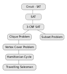

Some NP-complete problems, indicating the reductions typically used to prove their NP-completeness

An interesting example is the graph isomorphism problem, the graph theory problem of determining whether a graph isomorphism exists between two graphs. Two graphs are isomorphic if one can be transformed into the other simply by renaming vertices. Consider these two problems:

• Graph Isomorphism: Is graph G₁ isomorphic to graph G₂?
• Subgraph Isomorphism: Is graph G₁ isomorphic to a subgraph of graph G₂?

The Subgraph Isomorphism problem is NP-complete. The graph isomorphism problem is suspected to be neither in P nor NP-complete, though it is in NP. This is an example of a problem that is thought to be hard, but isn't thought to be NP-complete.

The easiest way to prove that some new problem is NP-complete is first to prove that it is in NP, and then to reduce some known NP-complete problem to it. Therefore, it is useful to know a variety of NP-complete problems. The list below contains some well-known problems that are NP-complete when expressed as decision problems.

• Boolean satisfiability problem (Sat.)
• N-puzzle
• Knapsack problem
• Hamiltonian path problem
• Travelling salesman problem
• Subgraph isomorphism problem
• Subset sum problem
• Clique problem
• Vertex cover problem
• Independent set problem
• Dominating set problem
• Graph coloring problem

To the right is a diagram of some of the problems and the reductions typically used to prove their NP-completeness. In this diagram, an arrow from one problem to another indicates the direction of the reduction. Note that this diagram is misleading as a description of the mathematical relationship between these problems, as there exists a polynomial-time reduction between any two NP-complete problems; but it indicates where demonstrating this polynomial-time reduction has been easiest.

There is often only a small difference between a problem in P and an NP-complete problem. For example, the 3-satisfiability problem, a restriction of the boolean satisfiability problem, remains NP-complete, whereas the slightly more restricted 2-satisfiability problem is in P (specifically, NL-complete), and the slightly more general max. 2-sat. problem is again NP-complete. Determining whether a graph can be colored with 2 colors is in P, but with 3 colors is NP-complete, even when restricted to planar graphs. Determining if a graph is a cycle or is bipartite is very easy (in L), but finding a maximum bipartite or a maximum cycle subgraph is NP-complete. A solution of the knapsack problem within any fixed percentage of the optimal solution can be computed in polynomial time, but finding the optimal solution is NP-complete.

Solving NP-complete problems

At present, all known algorithms for NP-complete problems require time that is superpolynomial in the input size, and it is unknown whether there are any faster algorithms.

The following techniques can be applied to solve computational problems in general, and they often give rise to substantially faster algorithms:

• Approximation: Instead of searching for an optimal solution, search for an "almost" optimal one.
• Randomization: Use randomness to get a faster average running time, and allow the algorithm to fail with some small probability. See Monte Carlo method.
• Restriction: By restricting the structure of the input (e.g., to planar graphs), faster algorithms are usually possible.
• Parameterization: Often there are fast algorithms if certain parameters of the input are fixed.
• Heuristic: An algorithm that works "reasonably well" in many cases, but for which there is no proof that it is both always fast and always produces a good result. Metaheuristic approaches are often used.

One example of a heuristic algorithm is a suboptimal $\scriptstyle O(n\log n)$ greedy coloring algorithm used for graph coloring during the register allocation phase of some compilers, a technique called graph-coloring global register allocation. Each vertex is a variable, edges are drawn between variables which are being used at the same time, and colors indicate the register assigned to each variable. Because most RISC machines have a fairly large number of general-purpose registers, even a heuristic approach is effective for this application.

Completeness under different types of reduction

In the definition of NP-complete given above, the term reduction was used in the technical meaning of a polynomial-time many-one reduction.

Another type of reduction is polynomial-time Turing reduction. A problem $\scriptstyle X$ is polynomial-time Turing-reducible to a problem $\scriptstyle Y$ if, given a subroutine that solves $\scriptstyle Y$ in polynomial time, one could write a program that calls this subroutine and solves $\scriptstyle X$ in polynomial time. This contrasts with many-one reducibility, which has the restriction that the program can only call the subroutine once, and the return value of the subroutine must be the return value of the program.

If one defines the analogue to NP-complete with Turing reductions instead of many-one reductions, the resulting set of problems won't be smaller than NP-complete; it is an open question whether it will be any larger.

Another type of reduction that is also often used to define NP-completeness is the logarithmic-space many-one reduction which is a many-one reduction that can be computed with only a logarithmic amount of space. Since every computation that can be done in logarithmic space can also be done in polynomial time it follows that if there is a logarithmic-space many-one reduction then there is also a polynomial-time many-one reduction. This type of reduction is more refined than the more usual polynomial-time many-one reductions and it allows us to distinguish more classes such as P-complete. Whether under these types of reductions the definition of NP-complete changes is still an open problem. All currently known NP-complete problems are NP-complete under log space reductions. Indeed, all currently known NP-complete problems remain NP-complete even under much weaker reductions.^[2] It is known, however, that AC⁰ reductions define a strictly smaller class than polynomial-time reductions.^[3]

Naming

According to Don Knuth, the name "NP-complete" was popularized by Alfred Aho, John Hopcroft and Jeffrey Ullman in their celebrated textbook "The Design and Analysis of Computer Algorithms". He reports that they introduced the change in the galley proofs for the book (from "polynomially-complete"), in accordance with the results of a poll he had conducted of the Theoretical Computer Science community.^[4] Other suggestions made in the poll^[5] included "Herculean", "formidable", Steiglitz's "hard-boiled" in honor of Cook, and Shen Lin's acronym "PET", which stood for "probably exponential time", but depending on which way the P versus NP problem went, could stand for "provably exponential time" or "previously exponential time".^[6]

Common misconceptions

The following misconceptions are frequent.^[7]

• "NP-complete problems are the most difficult known problems." Since NP-complete problems are in NP, their running time is at most exponential. However, some problems provably require more time, for example Presburger arithmetic.
• "NP-complete problems are difficult because there are so many different solutions." On the one hand, there are many problems that have a solution space just as large, but can be solved in polynomial time (for example minimum spanning tree). On the other hand, there are NP-problems with at most one solution that are NP-hard under randomized polynomial-time reduction (see Valiant–Vazirani theorem).
• "Solving NP-complete problems requires exponential time." First, this would imply P ≠ NP, which is still an unsolved question. Further, some NP-complete problems actually have algorithms running in superpolynomial, but subexponential time. For example, the Independent set and Dominating set problems are NP-complete when restricted to planar graphs, but can be solved in subexponential time on planar graphs using the planar separator theorem.
• "All instances of an NP-complete problem are difficult." Often some instances, or even almost all instances, may be easy to solve within polynomial time.

See also

• List of NP-complete problems
• Almost complete
• Ladner's theorem
• Strongly NP-complete
• P = NP problem
• NP-hard

References

1. ^ Garey, Michael R.; Johnson, D. S. (1979). Victor Klee. ed. Computers and Intractability: A Guide to the Theory of NP-Completeness. A Series of Books in the Mathematical Sciences. W. H. Freeman and Co.. pp. x+338. ISBN 0-7167-1045-5. MR519066. 
2. ^ Agrawal, M.; Allender, E.; Rudich, Steven (1998). "Reductions in Circuit Complexity: An Isomorphism Theorem and a Gap Theorem". Journal of Computer and System Sciences (Boston, MA: Academic Press) 57 (2): 127–143. doi:10.1006/jcss.1998.1583. ISSN 1090-2724 
3. ^ Agrawal, M.; Allender, E.; Impagliazzo, R.; Pitassi, T.; Rudich, Steven (2001). "Reducing the complexity of reductions". Computational Complexity (Birkhäuser Basel) 10 (2): 117–138. doi:10.1007/s00037-001-8191-1. ISSN 1016-3328 
4. ^ Don Knuth, Tracy Larrabee, and Paul M. Roberts, Mathematical Writing § 25, MAA Notes No. 14, MAA, 1989 (also Stanford Technical Report, 1987).
5. ^ Knuth, D. F. (1974). "A terminological proposal". SIGACT News 6 (1): 12–18. doi:10.1145/1811129.1811130. http://portal.acm.org/citation.cfm?id=1811130. Retrieved 2010-08-28. 
6. ^ See the poll, or [1].
7. ^ http://www.nature.com/news/2000/000113/full/news000113-10.html

• Garey, M.R.; Johnson, D.S. (1979). Computers and Intractability: A Guide to the Theory of NP-Completeness. New York: W.H. Freeman. ISBN 0-7167-1045-5.  This book is a classic, developing the theory, then cataloguing many NP-Complete problems.
• Cook, S.A. (1971). "The complexity of theorem proving procedures". Proceedings, Third Annual ACM Symposium on the Theory of Computing, ACM, New York. pp. 151–158. doi:10.1145/800157.805047. 
• Dunne, P.E. "An annotated list of selected NP-complete problems". COMP202, Dept. of Computer Science, University of Liverpool. http://www.csc.liv.ac.uk/~ped/teachadmin/COMP202/annotated_np.html. Retrieved 2008-06-21. 
• Crescenzi, P.; Kann, V.; Halldórsson, M.; Karpinski, M.; Woeginger, G. "A compendium of NP optimization problems". KTH NADA, Stockholm. http://www.nada.kth.se/~viggo/problemlist/compendium.html. Retrieved 2008-06-21. 
• Dahlke, K. "NP-complete problems". Math Reference Project. http://www.mathreference.com/lan-cx-np,intro.html. Retrieved 2008-06-21. 
• Karlsson, R. "Lecture 8: NP-complete problems" (PDF). Dept. of Computer Science, Lund University, Sweden. http://www.cs.lth.se/home/Rolf_Karlsson/bk/lect8.pdf. Retrieved 2008-06-21. ^{[dead link]}
• Sun, H.M. "The theory of NP-completeness" (PPT). Information Security Laboratory, Dept. of Computer Science, National Tsing Hua University, Hsinchu City, Taiwan. http://is.cs.nthu.edu.tw/course/2008Spring/cs431102/hmsunCh08.ppt. Retrieved 2008-06-21. 
• Jiang, J.R. "The theory of NP-completeness" (PPT). Dept. of Computer Science and Information Engineering, National Central University, Jhongli City, Taiwan. http://www.csie.ncu.edu.tw/%7Ejrjiang/alg2006/NPC-3.ppt. Retrieved 2008-06-21. 
• Cormen, T.H.; Leiserson, C.E., Rivest, R.L.; Stein, C. (2001). Introduction to Algorithms (2nd ed.). MIT Press and McGraw-Hill. Chapter 34: NP–Completeness, pp. 966–1021. ISBN 0-262-03293-7. 
• Sipser, M. (1997). Introduction to the Theory of Computation. PWS Publishing. Sections 7.4–7.5 (NP-completeness, Additional NP-complete Problems), pp. 248–271. ISBN 0-534-94728-X. 
• Papadimitriou, C. (1994). Computational Complexity (1st ed.). Addison Wesley. Chapter 9 (NP-complete problems), pp. 181–218. ISBN 0201530821. 
• Computational Complexity of Games and Puzzles
• Tetris is Hard, Even to Approximate
• Minesweeper is NP-complete!

Further reading

• Scott Aaronson, NP-complete Problems and Physical Reality, ACM SIGACT News, Vol. 36, No. 1. (March 2005), pp. 30–52.
• Lance Fortnow, The status of the P versus NP problem, Commun. ACM, Vol. 52, No. 9. (2009), pp. 78–86.