- Kinematics
-
Kinematics (from Greek κινεῖν, kinein, to move) is the branch of classical mechanics that describes the motion of bodies (objects) and systems (groups of objects) without consideration of the forces that cause the motion.[1][2][3][4]
Kinematics is not to be confused with another branch of classical mechanics: analytical dynamics (the study of the relationship between the motion of objects and its causes), sometimes subdivided into kinetics (the study of the relation between external forces and motion) and statics (the study of the relations in a system at equilibrium). Kinematics also differs from dynamics as used in modern-day physics to describe time-evolution of a system.
The term kinematics is less common today than in the past, but still has a role in physics.[5] (See analytical dynamics for more detail on usage). The term kinematics also finds use in biomechanics and animal locomotion.[6] Further, mathematicians that include time as a parameter in geometry have developed the subject of kinematic geometry.
The simplest application of kinematics is for particle motion, translational or rotational. The next level of complexity comes from the introduction of rigid bodies, which are collections of particles having time invariant distances between themselves. Rigid bodies might undergo translation and rotation or a combination of both. A more complicated case is the kinematics of a system of rigid bodies, which may be linked together by mechanical joints. Kinematics can be used to find the possible range of motion for a given mechanism, or, working in reverse, can be used to design a mechanism that has a desired range of motion. The movement of a crane and the oscillations of a piston in an engine are both simple kinematic systems. The crane is a type of open kinematic chain, while the piston is part of a closed four-bar linkage.
Contents
Linear motion
See also: Mechanics of planar particle motionLinear or translational kinematics[7][8] is the description of the motion in space of a point along a line, also known as a trajectory or path.[note 1] This path can be either straight (rectilinear) or curved (curvilinear).
Particle kinematics
Particle kinematics is the study of the kinematics of a single particle. The results obtained in particle kinematics are used to study the kinematics of collection of particles, dynamics and in many other branches of mechanics.
Position and reference frames
The position of a point in space is the most fundamental idea in particle kinematics. To specify the position of a point, one must specify three things: the reference point (often called the origin), distance from the reference point and the direction in space of the straight line from the reference point to the particle. Exclusion of any of these three parameters renders the description of position incomplete. Consider for example a tower 50 m south from your home. The reference point is home, the distance 50 m and the direction south. If one only says that the tower is 50 m south, the natural question that arises is "from where?" If one says that the tower is southward from your home, the question that arises is "how far?" If one says the tower is 50 m from your home, the question that arises is "in which direction?" Hence, all these three parameters are crucial to defining uniquely the position of a point in space.
Position is usually described by mathematical quantities that have all these three attributes: the most common are vectors and complex numbers. Usually, only vectors are used. For measurement of distances and directions, usually three dimensional coordinate systems are used with the origin coinciding with the reference point. A three-dimensional coordinate system (whose origin coincides with the reference point) with some provision for time measurement is called a reference frame or frame of reference or simply frame. All observations in physics are incomplete without the reference frame being specified.
Position vector
The position vector of a particle is a vector drawn from the origin of the reference frame to the particle. It expresses both the distance of the point from the origin and its sense from the origin. In three dimensions, the position of point A can be expressed as
where xA, yA, and zA are the Cartesian coordinates of the point. The magnitude of the position vector |r| gives the distance between the point A and the origin.
The direction cosines of the position vector provide a quantitative measure of direction. It is important to note that the position vector of a particle isn't unique. The position vector of a given particle is different relative to different frames of reference.
Rest and motion
Once the concept of position is firmly established, the ideas of rest and motion naturally follow. If the position vector of the particle (relative to a given reference frame) changes with time, then the particle is said to be in motion with respect to the chosen reference frame. However, if the position vector of the particle (relative to a given reference frame) remains the same with time, then the particle is said to be at rest with respect to the chosen frame. Note that rest and motion are relative to the reference frame chosen. It is quite possible that a particle at rest relative to a particular reference frame is in motion relative to the other. Hence, rest and motion aren't absolute terms, rather they are dependent on reference frame. For example, a passenger in a moving car may be at rest with respect to the car, but in motion with respect to the road.
Path
A particle's path is the locus between its beginning and end points which is reference-frame dependent. The path of a particle may be rectilinear (straight line) in one frame, and curved in another.
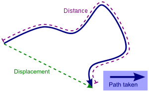
Displacement
Displacement is a vector describing the difference in position between two points, i.e. it is the change in position the particle undergoes during the time interval. If point A has position rA = (xA,yA,zA) and point B has position rB = (xB,yB,zB), the displacement rAB of B from A is given by
Geometrically, displacement is the shortest distance between the points A and B. Displacement, distinct from position vector, is independent of the reference frame. This can be understood as follows: the positions of points is frame dependent, however, the shortest distance between any pair of points is invariant on translation from one frame to another (barring relativistic cases).
 The distance traveled is always greater than or equal to the displacement.
Distance
Distance is a scalar quantity, describing the length of the path between two points along which a particle has travelled.
When considering the motion of a particle over time, distance is the length of the particle's path and may be different from displacement, which is the change from its initial position to its final position. For example, a race car traversing a 10 km closed loop from start to finish travels a distance of 10 km; its displacement, however, is zero because it arrives back at its initial position.
If the position of the particle is known as a function of time (r = r(t)), the distance s it travels from time t1 to time t2 can be found by
The formula utilizes the fact that over an infinitesimal time interval, the magnitude of the displacement equals the distance covered in that interval. This is analogous to the geometric fact that infinitesimal arcs on a curved line coincide with the chord drawn between the ends of the arc itself.
Velocity and speed
Average velocity is defined as
where Δr is the change in position and Δt is the interval of time over which the position changes. The direction of v is same as the direction of the change in position Δr as Δt>0.
Velocity is the measure of the rate of change in position with respect to time, that is, how the distance of a point changes with each instant of time. Velocity also is a vector. Instantaneous velocity (the velocity at an instant of time) can be defined as the limiting value of average velocity as the time interval Δt becomes smaller and smaller. Both Δr and Δt approach zero but the ratio v approaches a non-zero limit v. That is,
where dr is an infinitesimally small displacement and dt is an infinitesimally small length of time.[note 2] As per its definition in the derivative form, velocity can be said to be the time rate of change of position. Further, as dr is tangential to the actual path, so is the velocity.
As a position vector itself is frame dependent, velocity is also dependent on the reference frame.
The speed of an object is the magnitude |v| of its velocity. It is a scalar quantity:
The distance traveled by a particle over time is a non-decreasing quantity. Hence, ds/dt is non-negative, which implies that speed is also non-negative.
Acceleration
Average acceleration (acceleration over a length of time) is defined as:
where Δv is the change in velocity and Δt is the interval of time over which velocity changes.
Acceleration is the vector quantity describing the rate of change with time of velocity. Instantaneous acceleration (the acceleration at an instant of time) is defined as the limiting value of average acceleration as Δt becomes smaller and smaller. Under such a limit, a → a.
where dv is an infinitesimally small change in velocity and dt is an infinitesimally small length of time.
Types of motion based on velocity and acceleration
If the acceleration of a particle is zero, then the velocity of the particle is constant over time and the motion is said to be uniform. Otherwise, the motion is non-uniform.
If the acceleration is non-zero but constant, the motion is said to be motion with constant acceleration. On the other hand, if the acceleration is variable, the motion is called motion with variable acceleration. In motion with variable acceleration, the rate of change of acceleration is called the jerk.
Integral relations
The above definitions can be inverted by mathematical integration to find:
Kinematics of constant acceleration
Many physical situations can be modeled as constant-acceleration processes, such as projectile motion.
Integrating acceleration a with respect to time t gives the change in velocity. When acceleration is constant both in direction and in magnitude, the point is said to be undergoing uniformly accelerated motion. In this case, the integral relations can be simplified:
Additional relations between displacement, velocity, acceleration, and time can be derived. Since a = (v − v0)/t,
By using the definition of an average, this equation states that when the acceleration is constant average velocity times time equals displacement.
A relationship without explicit time dependence may also be derived for one-dimensional motion. Noting that at = v − v0,
where · denotes the dot product. Dividing the t on both sides and carrying out the dot-products:
In the case of straight-line motion, (r - r0) is parallel to a. Then
This relation is useful when time is not known explicitly.
Relative velocity
Main article: Relative velocityTo describe the motion of object A with respect to object B, when we know how each is moving with respect to a reference object O, we can use vector algebra. Choose an origin for reference, and let the positions of objects A, B, and O be denoted by rA, rB, and rO. Then the position of A relative to the reference object O is
Consequently, the position of A relative to B is
The above relative equation states that the motion of A relative to B is equal to the motion of A relative to O minus the motion of B relative to O. It may be easier to visualize this result if the terms are re-arranged:
or, in words, the motion of A relative to the reference is that of B plus the relative motion of A with respect to B. These relations between displacements become relations between velocities by simple time-differentiation, and a second differentiation makes them apply to accelerations.
For example, let Ann move with velocity
 relative to the reference (we drop the O subscript for convenience) and let Bob move with velocity
  , each velocity given with respect to the ground (point O). To find how fast Ann is moving relative to Bob (we call this velocity
  ), the equation above gives:
To find
we simply rearrange this equation to obtain:At velocities comparable to the speed of light, these equations are not valid. They are replaced by equations derived from Einstein's theory of special relativity.
-
Example: Rectilinear (1D) motion  Figure A: An object is fired upwards, reaches its apex, and then begins its descent under a constant acceleration. Note: The equations described here holds for object fired from ground and should not be mistaken with this picture.
Consider an object that is fired directly upwards and falls back to the ground so that its trajectory is contained in a straight line. If we adopt the convention that the upward direction is the positive direction, the object experiences a constant acceleration of approximately −9.81 m s−2. Therefore, its motion can be modeled with the equations governing uniformly accelerated motion.
For the sake of example, assume the object has an initial velocity of +50 m s−1. There are several interesting kinematic questions we can ask about the particle's motion:
- How long will it be airborne?
To answer this question, we apply the formula
Since the question asks for the length of time between the object leaving the ground and hitting the ground on its fall, the displacement is zero.
There are two solutions: the first, t = 0, is trivial. The solution of interest is
- What altitude will it reach before it begins to fall?
In this case, we use the fact that the object has a velocity of zero at the apex of its trajectory. Therefore, the applicable equation is:
If the origin of our coordinate system is at the ground, then xi is zero. Then we solve for xf and substitute known values:
- What will its final velocity be when it reaches the ground?
To answer this question, we use the fact that the object has an initial velocity of zero at the apex before it begins its descent. We can use the same equation we used for the last question, using the value of 127.55 m for xi.
Assuming this experiment were performed in a vacuum (negating drag effects), we find that the final and initial speeds are equal, a result which agrees with conservation of energy.
-
Example: Projectile (2D) motion  Figure B: An object fired at an angle θ from the ground follows a parabolic trajectory. Note: The equations described here holds for object fired from ground and should not be mistaken with this picture.
Suppose that an object is not fired vertically but is fired at an angle θ from the ground. The object will then follow a parabolic trajectory, and its horizontal motion can be modeled independently of its vertical motion. Assume that the object is fired at an initial velocity of 50 m s−1 and 30° from the horizontal.
- How far will it travel before hitting the ground?
The object experiences an acceleration of −9.81 m s−2 in the vertical direction and no acceleration in the horizontal direction. Therefore, the horizontal displacement is
Solving the equation requires finding t. This can be done by analyzing the motion in the vertical direction. If we impose that the vertical displacement is zero, we can use the same procedure we did for rectilinear motion to find t.
We now solve for t and substitute this expression into the original expression for horizontal displacement.
Note the use of the trigonometric identity 2sinθ cosθ = sin 2θ.
Kinematics is the study of how things move. Here, we are interested in the motion of normal objects in our world. A normal object is visible, has edges, and has a location that can be expressed with (x, y, z) coordinates. We will not be discussing the motion of atomic particles or black holes or light.
We will create a vocabulary and a group of mathematical methods that will describe this ordinary motion. Understand that we will be developing a language for describing motion only. We won't be concerned with what is causing or changing the motion, or more correctly, the momentums of the objects. In other words, we are not concerned with the action of forces within this topic.
Rotational motion
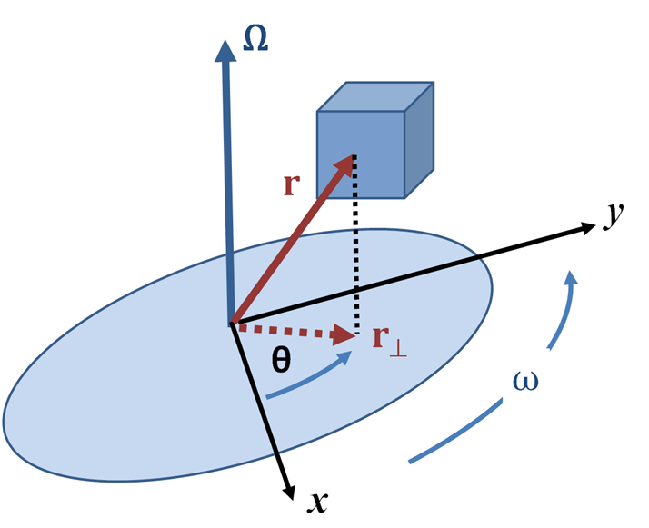
Main article: Circular motion Figure 1: The angular velocity vector Ω points up for counterclockwise rotation and down for clockwise rotation, as specified by the right-hand rule. Angular position θ(t) changes with time at a rate ω(t) = dθ/dt.
Rotational or angular kinematics is the description of the rotation of an object.[9] The description of rotation requires some method for describing orientation. Common descriptions include Euler angles and the kinematics of turns induced by algebraic products.
In what follows, attention is restricted to simple rotation about an axis of fixed orientation. The z-axis has been chosen for convenience.
Description of rotation then involves these three quantities:
- Angular position: The oriented distance from a selected origin on the rotational axis to a point of an object is a vector r ( t ) locating the point. The vector r(t) has some projection (or, equivalently, some component) r⊥(t) on a plane perpendicular to the axis of rotation. Then the angular position of that point is the angle θ from a reference axis (typically the positive x-axis) to the vector r⊥(t) in a known rotation sense (typically given by the right-hand rule).
- Angular velocity: The angular velocity ω is the rate at which the angular position θ changes with respect to time t:
The angular velocity is represented in Figure 1 by a vector Ω pointing along the axis of rotation with magnitude ω and sense determined by the direction of rotation as given by the right-hand rule.
- Angular acceleration: The magnitude of the angular acceleration α is the rate at which the angular velocity ω changes with respect to time t:
The equations of translational kinematics can easily be extended to planar rotational kinematics with simple variable exchanges:
Here θi and θf are, respectively, the initial and final angular positions, ωi and ωf are, respectively, the initial and final angular velocities, and α is the constant angular acceleration. Although position in space and velocity in space are both true vectors (in terms of their properties under rotation), as is angular velocity, angle itself is not a true vector.
Point object in circular motion
See also: Rigid body and Orientation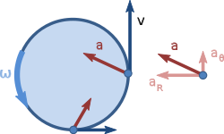 Figure 2: Velocity and acceleration for nonuniform circular motion: the velocity vector is tangential to the orbit, but the acceleration vector is not radially inward because of its tangential component aθ that increases the rate of rotation: dω/dt = |aθ|/R.
This example deals with a "point" object, by which is meant that complications due to rotation of the body itself about its own center of mass are ignored.
Displacement. An object in circular motion is located at a position r(t) given by:
where uR is a unit vector pointing outward from the axis of rotation toward the periphery of the circle of motion, located at a radius R from the axis.
Linear velocity. The velocity of the object is then
The magnitude of the unit vector uR (by definition) is fixed, so its time dependence is entirely due to its rotation with the radius to the object, that is,
where uθ is a unit vector perpendicular to uR pointing in the direction of rotation, ω(t) is the (possibly time varying) angular rate of rotation, and the symbol × denotes the vector cross product. The velocity is then:
The velocity therefore is tangential to the circular orbit of the object, pointing in the direction of rotation, and increasing in time if ω increases in time.
Linear acceleration. In the same manner, the acceleration of the object is defined as:
which shows a leading term aθ in the acceleration tangential to the orbit related to the angular acceleration of the object (supposing ω to vary in time) and a second term aR directed inward from the object toward the center of rotation, called the centripetal acceleration.
Coordinate systems
See also: Generalized coordinates, Curvilinear coordinates, Orthogonal coordinates, and Frenet-Serret formulasIn any given situation, the most useful coordinates may be determined by constraints on the motion, or by the geometrical nature of the force causing or affecting the motion. Thus, to describe the motion of a bead constrained to move along a circular hoop, the most useful coordinate may be its angle on the hoop. Similarly, to describe the motion of a particle acted upon by a central force, the most useful coordinates may be polar coordinates. Polar coordinates are extended into three dimensions with either the spherical polar or cylindrical polar coordinate systems. These are most useful in systems exhibiting spherical or cylindrical symmetry respectively.
Fixed rectangular coordinates
In this coordinate system, vectors are expressed as an addition of vectors in the x, y, and z direction from a non-rotating origin. Usually i, j, k are unit vectors in the x-, y-, and z-directions.
The position vector, r, the velocity vector, v, and the acceleration vector, a are expressed using rectangular coordinates in the following way:
Note:
 ,
, 
Two-dimensional rotating reference frame
See also: Centripetal forceThis coordinate system expresses only planar motion. It is based on three orthogonal unit vectors: the vector i, and the vector j which form a basis for the plane in which the objects we are considering reside, and k about which rotation occurs. Unlike rectangular coordinates, which are measured relative to an origin that is fixed and non-rotating, the origin of these coordinates can rotate and translate - often following a particle on a body that is being studied.
Derivatives of unit vectors
The position, velocity, and acceleration vectors of a given point can be expressed using these coordinate systems, but we have to be a bit more careful than we do with fixed frames of reference. Since the frame of reference is rotating, the unit vectors also rotate, and this rotation must be taken into account when taking the derivative of any of these vectors. If the coordinate frame is rotating at angular rate ω in the counterclockwise direction (that is, Ω = ω k using the right hand rule) then the derivatives of the unit vectors are as follows:
Position, velocity, and acceleration
Given these identities, we can now figure out how to represent the position, velocity, and acceleration vectors of a particle using this reference frame.
Position
Position is straightforward:
It is just the distance from the origin in the direction of each of the unit vectors.
Velocity
Velocity is the time derivative of position:
By the product rule, this is:
Which from the identities above we know to be:
or equivalently
where vrel is the velocity of the particle relative to the rotating coordinate system.
Acceleration
Acceleration is the time derivative of velocity.
We know that:
Consider the

 part. has two parts we want to find the derivative of: the relative change in velocity (
 ), and the change in the coordinate frame
(
 ).
).Next, consider
 . Using the chain rule:
 from above:
So all together:
And collecting terms:[10]
Kinematic constraints
A kinematic constraint is any condition relating properties of a dynamic system that must hold true at all times. Below are some common examples:
Rolling without slipping
An object that rolls against a surface without slipping obeys the condition that the velocity of its center of mass is equal to the cross product of its angular velocity with a vector from the point of contact to the center of mass,
 .
.
For the case of an object that does not tip or turn, this reduces to v = R ω.
Inextensible cord
This is the case where bodies are connected by an idealized cord that remains in tension and cannot change length. The constraint is that the sum of lengths of all segments of the cord is the total length, and accordingly the time derivative of this sum is zero. See Kelvin and Tait[11][12] and Fogiel.[13] A dynamic problem of this type is the pendulum. Another example is a drum turned by the pull of gravity upon a falling weight attached to the rim by the inextensible cord.[14] An equilibrium problem (not kinematic) of this type is the catenary.[15]
See also
- Acceleration
- Analytical mechanics
- Applied mechanics
- Celestial mechanics
- Centripetal force
- Chebychev–Grübler–Kutzbach criterion
- Classical mechanics
- Crackle (physics)
- Distance
- Dynamics (physics)
- Engineering
- Fictitious force
- Forward kinematics
- Four-bar linkage
- Inverse kinematics
- Jerk (physics)
- Jounce
- Kepler's laws
- Kinematic coupling
- Kinetics (physics)
- Motion
- Orbital mechanics
- Statics
- Velocity
Notes
- ^ In mathematics, a line refers to a straight trajectory, and a curve to a trajectory which may have curvature. In mechanics and kinematics, "line' and "curve" both refer to any trajectory, in particular a line may be a complex curve in space. Any position along a specified trajectory can be described by a single coordinate, the distance traversed along the path, or arc length. The motion of a particle along a trajectory can be described by specifying the time dependence of its position, for example by specification of the arc length locating the particle at each time t. The following words refer to curves and lines:
- "linear" (= along a straight or curved line;
- "rectilinear" (= along a straight line, from Latin rectus = straight, and linere = spread),
- "curvilinear" (=along a curved line, from Latin curvus = curved, and linere = spread).
- ^ Because magnitude of dr is necessarily the distance between two infinitesimally spaced points along the trajectory of the point, it is the same as an increment in arc length along the path of the point, customarily denoted ds.
References
- Moon, Francis C. (2007). The Machines of Leonardo Da Vinci and Franz Reuleaux, Kinematics of Machines from the Renaissance to the 20th Century. Springer. ISBN 9781402055980.
- ^ Edmund Taylor Whittaker & William McCrea (1988). A Treatise on the Analytical Dynamics of Particles and Rigid Bodies. Cambridge University Press. Chapter 1. ISBN 0521358833. http://books.google.com/books?id=epH1hCB7N2MC&printsec=frontcover&dq=inauthor:%22E+T+Whittaker%22&lr=&as_brr=0&sig=SN7_oYmNYM4QRSgjULXBU5jeQrA&source=gbs_book_other_versions_r&cad=0_2#PPA1,M1.
- ^ Joseph Stiles Beggs (1983). Kinematics. Taylor & Francis. p. 1. ISBN 0891163557. http://books.google.com/books?id=y6iJ1NIYSmgC&printsec=frontcover&dq=kinematics&lr=&as_brr=0&sig=brRJKOjqGTavFsydCzhiB3u_8MA#PPA1,M1.
- ^ O. Bottema & B. Roth (1990). Theoretical Kinematics. Dover Publications. reface. ISBN 0486663469. http://books.google.com/books?id=f8I4yGVi9ocC&printsec=frontcover&dq=kinematics&lr=&as_brr=0&sig=YfoHn9ImufIzAEp5Kl7rEmtYBKc#PPR7,M1.
- ^ Thomas Wallace Wright (1896). Elements of Mechanics Including Kinematics, Kinetics and Statics. E and FN Spon. Chapter 1. http://books.google.com/books?id=-LwLAAAAYAAJ&printsec=frontcover&dq=mechanics+kinetics&lr=&as_brr=0#PPA6,M1.
- ^ See, for example: Russell C. Hibbeler (2009). "Kinematics and kinetics of a particle". Engineering Mechanics: Dynamics (12th ed.). Prentice Hall. p. 298. ISBN 0136077919. http://books.google.com/books?id=tOFRjXB-XvMC&pg=PA298., Ahmed A. Shabana (2003). "Reference kinematics". Dynamics of Multibody Systems (2nd ed.). Cambridge University Press. ISBN 0521544114. http://books.google.com/books?id=zxuG-l7J5rgC&pg=PA28., P. P. Teodorescu (2007). "Kinematics". Mechanical Systems, Classical Models: Particle Mechanics. Springer. p. 287. ISBN 1402054416. http://books.google.com/books?id=k4H2AjWh9qQC&pg=PA287.
- ^ A. Biewener (2003). Animal Locomotion. Oxford University Press. ISBN 19850022X. http://books.google.com/books?id=yMaN9pk8QJAC.
- ^ James R. Ogden & Max Fogiel (1980). The Mechanics Problem Solver. Research and Education Association. p. 184. ISBN 0878915192. http://books.google.com/books?id=XVyD9pJpW-cC&pg=PA184&dq=%22curvilinear+kinematics%22&lr=&as_brr=0&sig=WW7us4UJzSWOA19pfdAbwTJvPR4.
- ^ R. Douglas Gregory (2006). Classical Mechanics: An Undergraduate Text. Cambridge UK: Cambridge University Press. Chapter 2. ISBN 0521826780. http://books.google.com/books?id=uAfUQmQbzOkC&printsec=frontcover&dq=%22rigid+body+kinematics%22&lr=&as_brr=0#PRA1-PA25,M1.
- ^ R. Douglas Gregory (2006). Chapter 16. Cambridge: Cambridge University. ISBN 0521826780. http://books.google.com/books?id=uAfUQmQbzOkC&printsec=frontcover&dq=%22rigid+body+kinematics%22&lr=&as_brr=0#PRA1-PA457,M1.
- ^ R. Douglas Gregory (2006). pp. 475-476. Cambridge: Cambridge University. ISBN 0521826780. http://books.google.com/books?id=uAfUQmQbzOkC&printsec=frontcover&dq=%22rigid+body+kinematics%22&lr=&as_brr=0#PRA1-PA475,M1.
- ^ William Thomson Kelvin & Peter Guthrie Tait (1894). Elements of Natural Philosophy. Cambridge University Press. p. 4. ISBN 1573929840. http://books.google.com/books?id=dHASAAAAIAAJ&pg=PA4&dq=%22inextensible+cord%22&lr=&as_brr=0&as_pt=ALLTYPES.
- ^ William Thomson Kelvin & Peter Guthrie Tait (1894). op. cit.. p. 296. http://books.google.com/books?id=ahtWAAAAMAAJ&pg=PA296&dq=%22inextensible+cord%22&lr=&as_brr=0&as_pt=ALLTYPES#PPA296,M1.
- ^ M. Fogiel (1980). "Problem 17-11". The Mechanics Problem Solver. Research & Education Assoc.. p. 613. ISBN 0878915192. http://books.google.com/books?id=XVyD9pJpW-cC&pg=PA613&dq=%22inextensible+cord%22&lr=&as_brr=0&as_pt=ALLTYPES.
- ^ Irving Porter Church (1908). Mechanics of Engineering. Wiley. p. 111. ISBN 1110365276. http://books.google.com/books?id=7-40AAAAMAAJ&pg=PA111&dq=%22inextensible+cord%22&lr=&as_brr=0&as_pt=ALLTYPES.
- ^ Morris Kline (1990). Mathematical Thought from Ancient to Modern Times. Oxford University Press. p. 472. ISBN 0195061365. http://books.google.com/books?id=aO-v3gvY-I8C&pg=PA472&dq=%22inextensible+cord%22&lr=&as_brr=0&as_pt=ALLTYPES.
External links
- Java applet of 1D kinematics
- Flash animated tutorial for 1D kinematics
- Physclips: Mechanics with animations and video clips from the University of New South Wales
- physicsfunda.googlepages.com, Kinematics for High School ant IIT JEE level
- Kinematic Models for Design Digital Library (KMODDL)
Movies and photos of hundreds of working mechanical-systems models at Cornell University. Also includes an e-book library of classic texts on mechanical design and engineering.
Kinematics ← Integrate … Differentiate →
Displacement (Distance) | Velocity (Speed) | Acceleration | Jerk | Jounce

kinemetics in also a branch of physics
Categories:


![\begin{align}
\mathbf{r}(t) &=\mathbf{r}_0 + \int_{t_0}^t \mathbf{v}(t) \; dt \\
&= \mathbf{r}_0 + \mathbf{v}_0 t + \int_{t_0}^t \left[\int_{t_0}^{t} \mathbf{a}(t) dt \right]\; dt \\
\end{align}](9/f89432078b57e8d6c20e944dcf772649.png)


Wikimedia Foundation. 2010.