Electrical impedance

Electromagnetism
Electricity · Magnetism
Electrostatics Electric charge · Coulomb's law · Electric field · Electric flux · Gauss's law · Electric potential energy · Electric potential · Electrostatic induction · Electric dipole moment · Polarization density
Magnetostatics Ampère's law · Electric current · Magnetic field · Magnetization · Magnetic flux · Biot–Savart law · Magnetic dipole moment · Gauss's law for magnetism
Electrodynamics Lorentz force law · emf · Electromagnetic induction · Faraday’s law · Lenz's law · Displacement current · Maxwell's equations · EM field · Electromagnetic radiation · Liénard–Wiechert potential · Maxwell tensor · Eddy current
Electrical Network Electrical conduction · Electrical resistance · Capacitance · Inductance · Impedance · Resonant cavities · Waveguides
Covariant formulation Electromagnetic tensor · EM Stress-energy tensor · Four-current · Electromagnetic four-potential
Scientists Ampère · Coulomb · Faraday · Gauss · Heaviside · Henry · Hertz · Lorentz · Maxwell · Tesla · Volta · Weber · Ørsted
v · d · e

A graphical representation of the complex impedance plane

Electrical impedance, or simply impedance, is the measure of the opposition that an electrical circuit presents to the passage of a current when a voltage is applied. In quantitative terms, it is the complex ratio of the voltage to the current in an alternating current (AC) circuit. Impedance extends the concept of resistance to AC circuits, and possesses both magnitude and phase, unlike resistance which has only magnitude. When a circuit is driven with direct current (DC), there is no distinction between impedance and resistance; the latter can be thought of as impedance with zero phase angle.

It is necessary to introduce the concept of impedance in AC circuits because there are other mechanisms impeding the flow of current besides the normal resistance of DC circuits. There are an additional two impeding mechanisms to be taken into account in AC circuits: the induction of voltages in conductors self-induced by the magnetic fields of currents (inductance), and the electrostatic storage of charge induced by voltages between conductors (capacitance). The impedance caused by these two effects is collectively referred to as reactance and forms the imaginary part of complex impedance whereas resistance forms the real part.

The symbol for impedance is usually $\scriptstyle Z$ and it may be represented by writing its magnitude and phase in the form $\scriptstyle |Z| \angle \theta$. However, complex number representation is often more powerful for circuit analysis purposes. The term impedance was coined by Oliver Heaviside in July 1886.^[1][2] Arthur Kennelly was the first to represent impedance with complex numbers in 1893.^[3]

Impedance is defined as the frequency domain ratio of the voltage to the current.^[4] In other words, it is the voltage–current ratio for a single complex exponential at a particular frequency ω. In general, impedance will be a complex number, with the same units as resistance, for which the SI unit is the ohm (Ω). For a sinusoidal current or voltage input, the polar form of the complex impedance relates the amplitude and phase of the voltage and current. In particular,

• The magnitude of the complex impedance is the ratio of the voltage amplitude to the current amplitude.
• The phase of the complex impedance is the phase shift by which the current is ahead of the voltage.

The reciprocal of impedance is admittance (i.e., admittance is the current-to-voltage ratio, and it conventionally carries units of siemens, formerly called mhos).

Complex impedance

Impedance is represented as a complex quantity $\scriptstyle Z$ and the term complex impedance may be used interchangeably; the polar form conveniently captures both magnitude and phase characteristics,

$\ Z = |Z| e^{j\theta} \quad$

where the magnitude $\scriptstyle |Z|$ represents the ratio of the voltage difference amplitude to the current amplitude, while the argument $\scriptstyle \theta$ gives the phase difference between voltage and current and $\scriptstyle j$ is the imaginary unit. In Cartesian form,

$\ Z = R + jX \quad$

where the real part of impedance is the resistance $\scriptstyle R$ and the imaginary part is the reactance $\scriptstyle X$.

Where it is required to add or subtract impedances the cartesian form is more convenient, but when quantities are multiplied or divided the calculation becomes simpler if the polar form is used. A circuit calculation, such as finding the total impedance of two impedances in parallel, may require conversion between forms several times during the calculation. Conversion between the forms follows the normal conversion rules of complex numbers.

Ohm's law

An AC supply applying a voltage $\scriptstyle V$, across a load $\scriptstyle Z$, driving a current $\scriptstyle I$.

Main article: Ohm's law

The meaning of electrical impedance can be understood by substituting it into Ohm's law.^[5][6]

$\ V = I Z = I |Z| e^{j\theta} \quad$

The magnitude of the impedance $\scriptstyle |Z|$ acts just like resistance, giving the drop in voltage amplitude across an impedance $\scriptstyle Z$ for a given current $\scriptstyle I$. The phase factor tells us that the current lags the voltage by a phase of $\scriptstyle \theta$ (i.e. in the time domain, the current signal is shifted $\scriptstyle \frac{\theta}{2 \pi} T$ later with respect to the voltage signal).

Just as impedance extends Ohm's law to cover AC circuits, other results from DC circuit analysis such as voltage division, current division, Thevenin's theorem, and Norton's theorem, can also be extended to AC circuits by replacing resistance with impedance.

Complex voltage and current

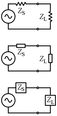Generalized impedances in a circuit can be drawn with the same symbol as a resistor (US ANSI or DIN Euro) or with a labeled box.

In order to simplify calculations, sinusoidal voltage and current waves are commonly represented as complex-valued functions of time denoted as $\scriptstyle V$ and $\scriptstyle I$.^[7][8]

$\ V = |V|e^{j(\omega t + \phi_V)}$

$\ I = |I|e^{j(\omega t + \phi_I)}$

Impedance is defined as the ratio of these quantities.

$\ Z = \frac{V}{I}$

Substituting these into Ohm's law we have

$\begin{align} |V| e^{j(\omega t + \phi_V)} &= |I| e^{j(\omega t + \phi_I)} |Z| e^{j\theta} \\ &= |I| |Z| e^{j(\omega t + \phi_I + \theta)} \end{align}$

Noting that this must hold for all t, we may equate the magnitudes and phases to obtain

$\ |V| = |I| |Z| \quad$

$\ \phi_V = \phi_I + \theta \quad$

The magnitude equation is the familiar Ohm's law applied to the voltage and current amplitudes, while the second equation defines the phase relationship.

Validity of complex representation

This representation using complex exponentials may be justified by noting that (by Euler's formula):

$\ \cos(\omega t + \phi) = \frac{1}{2} \Big[ e^{j(\omega t + \phi)} + e^{-j(\omega t + \phi)}\Big]$

i.e. a real-valued sinusoidal function (which may represent our voltage or current waveform) may be broken into two complex-valued functions. By the principle of superposition, we may analyse the behaviour of the sinusoid on the left-hand side by analysing the behaviour of the two complex terms on the right-hand side. Given the symmetry, we only need to perform the analysis for one right-hand term; the results will be identical for the other. At the end of any calculation, we may return to real-valued sinusoids by further noting that

$\ \cos(\omega t + \phi) = \Re \Big\{ e^{j(\omega t + \phi)} \Big\}$

In other words, we simply take the real part of the result.

Phasors

Main article: Phasor (electronics)

A phasor is a constant complex number, usually expressed in exponential form, representing the complex amplitude (magnitude and phase) of a sinusoidal function of time. Phasors are used by electrical engineers to simplify computations involving sinusoids, where they can often reduce a differential equation problem to an algebraic one.

The impedance of a circuit element can be defined as the ratio of the phasor voltage across the element to the phasor current through the element, as determined by the relative amplitudes and phases of the voltage and current. This is identical to the definition from Ohm's law given above, recognising that the factors of $\scriptstyle e^{j\omega t}$ cancel.

Device examples

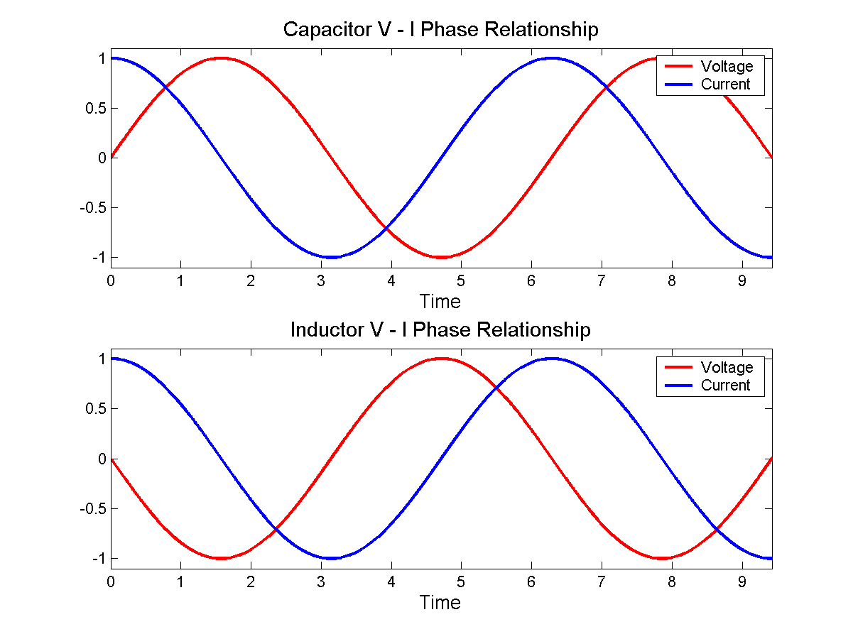
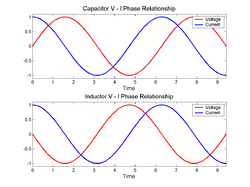The phase angles in the equations for the impedance of inductors and capacitors indicate that the voltage across a capacitor lags the current through it by a phase of π / 2, while the voltage across an inductor leads the current through it by π / 2. The identical voltage and current amplitudes tell us that the magnitude of the impedance is equal to one.

The impedance of an ideal resistor is purely real and is referred to as a resistive impedance:

$\ Z_R = R.$

In this case the voltage and current waveforms are proportional and in phase.

Ideal inductors and capacitors have a purely imaginary reactive impedance:

$\ Z_L = j\omega L,$

the impedance of inductors increases with frequency;

$\ Z_C = \frac{1}{j\omega C},$

the impedance of capacitors decreases with frequency.

In both cases, for an applied sinusoidal voltage, the resulting current is also sinusoidal, but in quadrature, 90 degrees out of phase with the voltage. However the phases have opposite signs: in an inductor, the current is lagging; in a capacitor the current is leading.

Note the following identities for the imaginary unit and its reciprocal:

$j = \cos{\left(\frac{\pi}{2}\right)} + j\sin{\left(\frac{\pi}{2}\right)} = e^{j\frac{\pi}{2}},$

$\frac{1}{j} = -j = \cos{\left(-\frac{\pi}{2}\right)} + j\sin{\left(-\frac{\pi}{2}\right)} = e^{j(-\frac{\pi}{2})}.$

Thus we can rewrite the inductor and capacitor impedance equations in polar form:

$\ Z_L = \omega Le^{j\frac{\pi}{2}},$

$\ Z_C = \frac{1}{\omega C}e^{j(-\frac{\pi}{2})}.$

The magnitude tells us the change in voltage amplitude for a given current amplitude through the impedance, while the exponential factors give the phase relationship.

Deriving the device specific impedances

What follows below is a derivation of impedance for each of the three basic circuit elements, the resistor, the capacitor, and the inductor. Although the idea can be extended to define the relationship between the voltage and current of any arbitrary signal, these derivations will assume sinusoidal signals, since any arbitrary signal can be approximated as a sum of sinusoids through Fourier Analysis.

Resistor

For a resistor, we have the relation:

$v_{\text{R}} \left( t \right) = {i_{\text{R}} \left( t \right)}R.$

This is simply a statement of Ohm's Law.

Considering the voltage signal to be

$v_{\text{R}}(t) = V_p \sin(\omega t) \, ,$

it follows that

$\frac{v_{\text{R}} \left( t \right)}{i_{\text{R}} \left( t \right)} = \frac{V_p \sin(\omega t)}{I_p \sin \left( \omega t \right)} = R.$

This tells us that the ratio of AC voltage amplitude to AC current amplitude across a resistor is $\scriptstyle R$, and that the AC voltage leads the AC current across a resistor by 0 degrees.

This result is commonly expressed as

$Z_{\text{resistor}} = R \, .$

Capacitor

For a capacitor, we have the relation:

$i_{\text{C}}(t) = C \frac{\operatorname{d}v_{\text{C}}(t)}{\operatorname{d}t}.$

Considering the voltage signal to be

$v_{\text{C}}(t) = V_p \sin(\omega t) \,$

it follows that

$\frac{\operatorname{d}v_{\text{C}}(t)}{\operatorname{d}t} = \omega V_p \cos \left( \omega t \right).$

And thus

$\frac{v_{\text{C}} \left( t \right)}{i_{\text{C}} \left( t \right)} = \frac{V_p \sin(\omega t)}{\omega V_p C \cos \left( \omega t \right)}= \frac{\sin(\omega t)}{\omega C \sin \left( \omega t + \frac{\pi}{2}\right)}.$

This tells us that the ratio of AC voltage amplitude to AC current amplitude across a capacitor is $\scriptstyle \frac{1}{\omega C}$, and that the AC voltage lags the AC current across a capacitor by -90 degrees (or the AC current leads the AC voltage across a capacitor by 90 degrees).

This result is commonly expressed in polar form, as

$\ Z_{\text{capacitor}} = \frac{1}{\omega C} e^{-j \frac{\pi}{2}}$

or, by applying Euler's formula, as

$\ Z_{\text{capacitor}} = -j\frac{1}{\omega C} = \frac{1}{j \omega C} \, .$

Inductor

For the inductor, we have the relation:

$v_{\text{L}}(t) = L \frac{\operatorname{d}i_{\text{L}}(t)}{\operatorname{d}t}.$

This time, considering the current signal to be

$i_{\text{L}}(t) = I_p \sin(\omega t) \, ,$

it follows that

$\frac{\operatorname{d}i_{\text{L}}(t)}{\operatorname{d}t} = \omega I_p \cos \left( \omega t \right).$

And thus

$\frac{v_{\text{L}} \left( t \right)}{i_{\text{L}} \left( t \right)} = \frac{\omega I_p L \cos(\omega t)}{I_p \sin \left( \omega t \right)}= \frac{\omega L \sin \left( \omega t + \frac{\pi}{2}\right)}{\sin(\omega t)}.$

This tells us that the ratio of AC voltage amplitude to AC current amplitude across an inductor is $\scriptstyle \omega L$, and that the AC voltage leads the AC current across an inductor by 90 degrees.

This result is commonly expressed in polar form, as

$\ Z_{\text{inductor}} = \omega L e^{j \frac{\pi}{2}} .$

Or, more simply, using Euler's formula, as

$\ Z_{\text{inductor}} = j \omega L. \,$

Generalised s-plane impedance

Impedance defined in terms of jω can strictly only be applied to circuits which are energised with a steady-state AC signal. The concept of impedance can be extended to a circuit energised with any arbitrary signal by using complex frequency instead of jω. Complex frequency is given the symbol s and is, in general, a complex number. Signals are expressed in terms of complex frequency by taking the Laplace transform of the time domain expression of the signal. The impedance of the basic circuit elements in this more general notation is as follows:

Element	Impedance expression
Resistor	$R \,$
Inductor	$sL \,$
Capacitor	$\frac{1}{sC} \,$

For a DC circuit this simplifies to s = 0. For a steady-state sinusoidal AC signal s = jω.

Resistance vs reactance

Resistance and reactance together determine the magnitude and phase of the impedance through the following relations:

$|Z| = \sqrt{Z Z^*} = \sqrt{R^2 + X^2}$

$\theta = \arctan{\left(\frac{X}{R}\right)}$

In many applications the relative phase of the voltage and current is not critical so only the magnitude of the impedance is significant.

Resistance

Main article: Electrical resistance

Resistance $\scriptstyle R$ is the real part of impedance; a device with a purely resistive impedance exhibits no phase shift between the voltage and current.

$\ R = |Z| \cos{\theta} \quad$

Reactance

Main article: Electrical reactance

Reactance $\scriptstyle X$ is the imaginary part of the impedance; a component with a finite reactance induces a phase shift $\scriptstyle \theta$ between the voltage across it and the current through it.

$\ X = |Z| \sin{\theta} \quad$

A purely reactive component is distinguished by the fact that the sinusoidal voltage across the component is in quadrature with the sinusoidal current through the component. This implies that the component alternately absorbs energy from the circuit and then returns energy to the circuit. A pure reactance will not dissipate any power.

Capacitive reactance

Main article: Capacitance

A capacitor has a purely reactive impedance which is inversely proportional to the signal frequency. A capacitor consists of two conductors separated by an insulator, also known as a dielectric.

$X_C = -(\omega C)^{-1} = -(2\pi f C)^{-1}\quad$

At low frequencies a capacitor is open circuit, as no charge flows in the dielectric. A DC voltage applied across a capacitor causes charge to accumulate on one side; the electric field due to the accumulated charge is the source of the opposition to the current. When the potential associated with the charge exactly balances the applied voltage, the current goes to zero.

Driven by an AC supply, a capacitor will only accumulate a limited amount of charge before the potential difference changes sign and the charge dissipates. The higher the frequency, the less charge will accumulate and the smaller the opposition to the current.

Inductive reactance

Main article: Inductance

Inductive reactance $\scriptstyle{X_L}$ is proportional to the signal frequency $\scriptstyle{f}$ and the inductance $\scriptstyle{L}$.

$X_L = \omega L = 2\pi f L\quad$

An inductor consists of a coiled conductor. Faraday's law of electromagnetic induction gives the back emf $\scriptstyle{\mathcal{E}}$ (voltage opposing current) due to a rate-of-change of magnetic flux density $\scriptstyle{B}$ through a current loop.

$\mathcal{E} = -{{d\Phi_B} \over dt}\quad$

For an inductor consisting of a coil with N loops this gives.

$\mathcal{E} = -N{d\Phi_B \over dt}\quad$

The back-emf is the source of the opposition to current flow. A constant direct current has a zero rate-of-change, and sees an inductor as a short-circuit (it is typically made from a material with a low resistivity). An alternating current has a time-averaged rate-of-change that is proportional to frequency, this causes the increase in inductive reactance with frequency.

Combining impedances

Main article: Series and parallel circuits

The total impedance of many simple networks of components can be calculated using the rules for combining impedances in series and parallel. The rules are identical to those used for combining resistances, except that the numbers in general will be complex numbers. In the general case however, equivalent impedance transforms in addition to series and parallel will be required.

Series combination

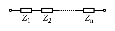
For components connected in series, the current through each circuit element is the same; the total impedance is simply the sum of the component impedances.

$\ Z_{\text{eq}} = Z_1 + Z_2 + \cdots + Z_n \quad$

Or explicitly in real and imaginary terms:

$\ Z_{\text{eq}} = R + jX = (R_1 + R_2 + \cdots + R_n) + j(X_1 + X_2 + \cdots + X_n) \quad$

Parallel combination

For components connected in parallel, the voltage across each circuit element is the same; the ratio of currents through any two elements is the inverse ratio of their impedances.

Hence the inverse total impedance is the sum of the inverses of the component impedances:

$\frac{1}{Z_{\text{eq}}} = \frac{1}{Z_1} + \frac{1}{Z_2} + \cdots + \frac{1}{Z_n}\,$

or, when n = 2:

$Z_{\text{eq}} = Z_1 \| Z_2 \,\stackrel{\text{def}}{=}\, \frac{Z_1 Z_2}{Z_1 + Z_2} \quad$

The equivalent impedance $\scriptstyle Z_{\text{eq}}$ can be calculated in terms of the equivalent resistance $\scriptstyle R_{\text{eq}}$ and reactance $\scriptstyle X_{\text{eq}}$.^[9]

$\ Z_{\text{eq}} = R_{\text{eq}} + j X_{\text{eq}} \quad$

$R_{\text{eq}} = \frac{(X_1 R_2 + X_2 R_1) (X_1 + X_2) + (R_1 R_2 - X_1 X_2) (R_1 + R_2)}{(R_1 + R_2)^2 + (X_1 + X_2)^2}$

$X_{\text{eq}} = \frac{(X_1 R_2 + X_2 R_1) (R_1 + R_2) - (R_1 R_2 - X_1 X_2) (X_1 + X_2)}{(R_1 + R_2)^2 + (X_1 + X_2)^2}$

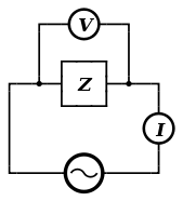
Measurement

The impedance of a device can be calculated by complex division of the voltage and current. The impedance of the device can be calculated by applying a sinusoidal voltage to the device in series with a resistor, and measuring the voltage across the resistor and across the device. Performing this measurement by sweeping the frequencies of the applied signal provides the impedance phase and magnitude.^[10]

Impulse impedance spectroscopy

The use of an impulse response may be used in combination with the fast Fourier transform (FFT) to rapidly measure the electrical impedance of various electrical devices. The technique compares well to other methodologies such as network and impedance analyzers while providing additional versatility in the electrical impedance measurement. The technique is theoretically simple, easy to implement and completed with ordinary laboratory instrumentation for minimal cost.^[10]

Variable impedance

In general, neither impedance nor admittance can be time varying as they are defined for complex exponentials for –∞ < t < +∞. If the complex exponential voltage–current ratio changes over time or amplitude, the circuit element cannot be described using the frequency domain. However, many systems (e.g., varicaps that are used in radio tuners) may exhibit non-linear or time-varying voltage–current ratios that appear to be LTI for small signals over small observation windows; hence, they can be roughly described as having a time-varying impedance. That is, this description is an approximation; over large signal swings or observation windows, the voltage–current relationship is non-LTI and cannot be described by impedance.

See also

• Impedance matching
• Impedance cardiography
• Impedance bridging
• Characteristic impedance
• Negative impedance converter
• Immittance

References

1. ^ Science, p. 18, 1888
2. ^ Oliver Heaviside, The Electrician, p. 212, 23 July 1886, reprinted as Electrical Papers, p 64, AMS Bookstore, ISBN 0821834657
3. ^ Kennelly, Arthur. Impedance (AIEE, 1893)
4. ^ Alexander, Charles; Sadiku, Matthew (2006). Fundamentals of Electric Circuits (3, revised ed.). McGraw-Hill. pp. 387–389. ISBN 9780073301150 
5. ^ AC Ohm's law, Hyperphysics
6. ^ Horowitz, Paul; Hill, Winfield (1989). "1". The Art of Electronics. Cambridge University Press. pp. 32–33. ISBN 0-521-37095-7. 
7. ^ Complex impedance, Hyperphysics
8. ^ Horowitz, Paul; Hill, Winfield (1989). "1". The Art of Electronics. Cambridge University Press. pp. 31–32. ISBN 0-521-37095-7. 
9. ^ Parallel Impedance Expressions, Hyperphysics
10. ^ ^{a b} Lewis Jr., George; George K. Lewis Sr. and William Olbricht (August 2008). "Cost-effective broad-band electrical impedance spectroscopy measurement circuit and signal analysis for piezo-materials and ultrasound transducers". Measurement Science and Technology 19 (10): 105102. Bibcode 2008MeScT..19j5102L. doi:10.1088/0957-0233/19/10/105102. PMC 2600501. PMID 19081773. http://www.iop.org/EJ/abstract/0957-0233/19/10/105102/. Retrieved 2008-09-15. 

External links

• Explaining Impedance
• Antenna Impedance
• ECE 209: Review of Circuits as LTI Systems – Brief explanation of Laplace-domain circuit analysis; includes a definition of impedance.