Permian–Triassic extinction event

K–T

Tr–J

P–Tr

Late D

O–S

Millions of years ago

The Permian–Triassic extinction event is the most significant extinction event in this plot for marine genera. (source and image info)

The Permian–Triassic (P–Tr) extinction event, informally known as the Great Dying,^[1] was an extinction event that occurred 251.4 Ma (million years) ago,^[2][3] forming the boundary between the Permian and Triassic geologic periods, as well as the Paleozoic and Mesozoic eras. It was the Earth's most severe extinction event, with up to 96% of all marine species^[4] and 70% of terrestrial vertebrate species becoming extinct.^[5] It is the only known mass extinction of insects.^[6][7] Some 57% of all families and 83% of all genera were killed. Because so much biodiversity was lost, the recovery of life on Earth took significantly longer than after other extinction events.^[4] This event has been described as the "mother of all mass extinctions."^[8]

Researchers have variously suggested that there were from one to three distinct pulses, or phases, of extinction.^{[2][5][9][10]} There are several proposed mechanisms for the extinctions; the earlier phase was likely due to gradual environmental change, while the latter phase has been argued to be due to a catastrophic event. Suggested mechanisms for the latter include large or multiple bolide impact events, increased volcanism, and sudden release of methane clathrate from the sea floor; gradual changes include sea-level change, anoxia, increasing aridity, and a shift in ocean circulation driven by climate change.^[11]

Dating the extinction

Permian–Triassic extinction

view • edit

-262 —

–

-260 —

–

-258 —

–

-256 —

–

-254 —

–

-252 —

–

-250 —

–

-248 —

–

-246 —

–

-244 —

–

-242 —

–

-240 —

–

-238 —

 

 

 

 

 

Induan

Olenekian

Anisian

Capitanian

Wuchia-
pingian

Chang-
hsingian

 

 

←

Extinction event

←

δ¹³C stabilises at +2 ‰. Calcified green algae return.^[12]

←

End-Guadalupian extinction pulse?

←

Full recovery of woody trees^[13]

←

Coals return^[14]

←

Scleractinian
corals & calcified sponges^[12]

P
e
r
m
i
a
n

T
r
i
a
s
s
i
c

 Mesozoic
 Palæozoic
 Lopingian (Upper Permian)
 Guadalupian (Middle Permian)

An approximate timescale of events around the P-Tr boundary.
Axis scale: millions of years ago.

PreЄ

Є

O

S

D

C

P

T

J

K

Pg

N

↓

Until 2000, it was thought that rock sequences spanning the Permian-Triassic boundary were too few and contained too many gaps for scientists to reliably determine its details.^[15] However, a study of uranium/lead ratios of zircons from rock sequences near Meishan in Changxing County of Zhejiang Province, China^[3] date the extinction to 251.4 ± 0.03 Ma, with an ongoing elevated extinction rate occurring for some time thereafter.^[2] A large ( approximately 9‰), abrupt global decrease in the ratio of ¹³C to ¹²C, denoted δ¹³C, coincides with this extinction,^{[13][16][17][18][19]} and is sometimes used to identify the Permian-Triassic boundary in rocks that are unsuitable for radiometric dating.^[20] Further evidence for environmental change around the P–Tr boundary suggests an 8 °C (14.40 °F) rise in temperature,^[13] and an increase in CO₂ levels by 2000ppm (by contrast, the concentration immediately before the industrial revolution was 280ppm;^[13] in October 2010, this concentration was 388 ppm, some 108 ppm higher^[21]). There is also evidence of increased ultraviolet radiation reaching the earth, and causing the mutation of plant spores.^[13]

It has been suggested that the Permian-Triassic boundary is associated with a sharp increase in the abundance of marine and terrestrial fungi, and that this was caused by the sharp increase in the amount of dead plants and animals fed upon by the fungi.^[22] For a while this "fungal spike" was used by some paleontologists to identify the Permian-Triassic boundary in rocks that are unsuitable for radiometric dating or lack suitable index fossils, but even the proposers of the fungal spike hypothesis pointed out that "fungal spikes" may have been a repeating phenomenon created by the post-extinction ecosystem in the earliest Triassic.^[22] More recently the very idea of a fungal spike has been criticized on several grounds, including that: Reduviasporonites, the most common supposed fungal spore, was actually a fossilized alga;^[13][23] the spike did not appear worldwide;^[24][25] and in many places it did not fall on the Permian-Triassic boundary.^[26] The algae, which were mis-identified as fungal spores, may even represent a transition to a lake-dominated Triassic world rather than an earliest Triassic zone of death and decay in some terrestrial fossil beds.^[27] However, newer chemical evidence agrees better with a fungal origin for Reduviasporonites, diluting these critiques.^[28]

Uncertainty exists regarding the duration of the overall extinction and about the timing and duration of various groups' extinctions within the greater process. Some evidence suggests that there were multiple extinction pulses^[5] or that the extinction was spread out over a few million years, with a very sharp peak in the last 1 million years of the Permian.^[26][29] Statistical analyses of some highly fossiliferous strata in Meishan, South China suggest that the main extinction was clustered around one peak.^[2] Recent research shows that different groups became extinct at different times; for example, while difficult to date absolutely, ostracod and brachiopod extinctions were separated by between 0.72 and 1.22 million years.^[30] In a well preserved sequence in east Greenland, the decline of animals is concentrated in a period 10 to 60 thousand years long, with plants taking several hundred thousand further years to show the full impact of the event.^[31] An older theory, still supported in some recent papers,^[32] is that there were two to three major extinction pulses 5 million years apart, separated by a period of extinctions well above the background level; and that the final extinction killed off only about 80% of marine species alive at that time while the other losses occurred during the first pulse or the interval between pulses. According to this theory one of these extinction pulses occurred at the end of the Guadalupian epoch of the Permian.^[5][33] For example, all but one of the surviving dinocephalian genera died out at the end of the Guadalupian,^[34] as did the Verbeekinidae, a family of large-size fusuline foraminifera.^[35] The impact of the end-Guadalupian extinction on marine organisms appears to have varied between locations and between taxonomic groups—brachiopods and corals had severe losses.^[36][37]

Extinction patterns

Marine extinctions	Genera extinct	Notes
Marine invertebrates
Foraminifera	97%	Fusulinids died out, but were almost extinct before the catastrophe
Radiolaria (plankton)	99%[38]
Anthozoa (sea anemones, corals, etc.)	96%	Tabulate and rugose corals died out
Bryozoans	79%	Fenestrates, trepostomes, and cryptostomes died out
Brachiopods	96%	Orthids and productids died out
Bivalves	59%
Gastropods (snails)	98%
Ammonites (cephalopods)	97%
Crinoids (echinoderms)	98%	Inadunates and camerates died out
Blastoids (echinoderms)	100%	May have become extinct shortly before the P–Tr boundary
Trilobites	100%	In decline since the Devonian; only 2 genera living before the extinction
Eurypterids ("sea scorpions")	100%	May have become extinct shortly before the P–Tr boundary
Ostracods (small crustaceans)	59%
Fish
Acanthodians	100%	In decline since the Devonian, with only one living family

Marine organisms

Marine invertebrates suffered the greatest losses during the P–Tr extinction. In the intensively-sampled south China sections at the P–Tr boundary, for instance, 286 out of 329 marine invertebrate genera disappear within the final 2 sedimentary zones containing conodonts from the Permian.^[2]

Statistical analysis of marine losses at the end of the Permian suggests that the decrease in diversity was caused by a sharp increase in extinctions instead of a decrease in speciation.^[39] The extinction primarily affected organisms with calcium carbonate skeletons, especially those reliant on ambient CO₂ levels to produce their skeletons.^[40]

Among benthic organisms, the extinction event multiplied background extinction rates, and therefore caused most damage to taxa that had a high background extinction rate (by implication, taxa with a high turnover).^[41][42] The extinction rate of marine organisms was catastrophic.^{[2][8][43][44]}

Surviving marine invertebrate groups include: articulate brachiopods (those with a hinge), which have suffered a slow decline in numbers since the P–Tr extinction; the Ceratitida order of ammonites; and crinoids ("sea lilies"), which very nearly became extinct but later became abundant and diverse.

The groups with the highest survival rates generally had active control of circulation, elaborate gas exchange mechanisms, and light calcification; more heavily calcified organisms with simpler breathing apparatus were the worst hit.^[12][45] In the case of the brachiopods at least, surviving taxa were generally small, rare members of a diverse community.^[46]

The ammonoids, which had been in a long-term decline for the 30 million years since the Roadian (middle Permian), suffered a selective end-Guadalupian extinction pulse. This extinction greatly reduced disparity, and suggests that environmental factors were responsible for this extinction. Diversity and disparity fell further until the P–Tr boundary; the extinction here was non-selective, consistent with a catastrophic initiator. During the Triassic, diversity rose rapidly, but disparity remained low.^[47]

The range of morphospace occupied by the ammonoids became more restricted as the Permian progressed. Just a few million years into the Triassic, the original morphospace range was once again occupied, but shared differently between clades.^[48]

Terrestrial invertebrates

The Permian had great diversity in insect and other invertebrate species, including the largest insects ever to have existed. The end-Permian is the only known mass extinction of insects,^[6] with eight or nine insect orders becoming extinct and ten more greatly reduced in diversity. Palaeodictyopteroids (insects with piercing and sucking mouthparts) began to decline during the mid-Permian; these extinctions have been linked to a change in flora. The greatest decline, however, occurred in the Late Permian and were probably not directly caused by weather-related floral transitions.^[8]

Most fossil insect groups found after the Permian–Triassic boundary differ significantly from those that lived prior to the P–Tr extinction. With the exception of the Glosselytrodea, Miomoptera, and Protorthoptera, Paleozoic insect groups have not been discovered in deposits dating to after the P–Tr boundary. The caloneurodeans, monurans, paleodictyopteroids, protelytropterans, and protodonates became extinct by the end of the Permian. In well-documented Late Triassic deposits, fossils overwhelmingly consist of modern fossil insect groups.^[6]

Terrestrial plants

Plant ecosystem response

The geological record of terrestrial plants is sparse, and based mostly on pollen and spore studies. Interestingly, plants are relatively immune to mass extinction, with the impact of all the major mass extinctions "negligible" at a family level.^[13] Even the reduction observed in species diversity (of 50%) may be mostly due to taphonomic processes.^[13] However, a massive rearrangement of ecosystems does occur, with plant abundances and distributions changing profoundly;^[13] the Palaeozoic flora scarcely survived this extinction.^[49]

At the P–Tr boundary, the dominant floral groups changed, with many groups of land plants entering abrupt decline, such as Cordaites (gymnosperms) and Glossopteris (seed ferns).^[50] Dominant gymnosperm genera were replaced post-boundary by lycophytes—extant lycophytes are recolonizers of disturbed areas.^[51]

Palynological or pollen studies from East Greenland of sedimentary rock strata laid down during the extinction period indicate dense gymnosperm woodlands before the event. At the same time that marine invertebrate macrofauna are in decline these large woodlands die out and are followed by a rise in diversity of smaller herbaceous plants including Lycopodiophyta, both Selaginellales and Isoetales. Later on other groups of gymnosperms again become dominant but again suffer major die offs; these cyclical flora shifts occur a few times over the course of the extinction period and afterwards. These fluctuations of the dominant flora between woody and herbaceous taxa indicate chronic environmental stress resulting in a loss of most large woodland plant species. The successions and extinctions of plant communities do not coincide with the shift in δ¹³C values, but occurs many years after.^[52] The recovery of gymnosperm forests took 4–5 million years.^[13]

Coal gap

No coal deposits are known from the Early Triassic, and those in the Middle Triassic are thin and low-grade.^[14] This "coal gap" has been explained in many ways. It has been suggested that new, more aggressive fungi, insects and vertebrates evolved, and killed vast numbers of trees. However these decomposers themselves suffered heavy losses of species during the extinction, and are not considered a likely cause of the coal gap.^[14] It could simply be that all coal forming plants were rendered extinct by the P–Tr extinction, and that it took 10 million years for a new suite of plants to adapt to the moist, acid conditions of peat bogs.^[14] On the other hand, abiotic factors (not caused by organisms), such as decreased rainfall or increased input of clastic sediments, may also be to blame.^[13] Finally, it is also true that there are very few sediments of any type known from the Early Triassic, and the lack of coal may simply reflect this scarcity. This opens the possibility that coal-producing ecosystems may have responded to the changed conditions by relocating, perhaps to areas where we have no sedimentary record for the Early Triassic.^[13] For example, in eastern Australia a cold climate had been the norm for a long period of time, with a peat mire ecosystem specialising to these conditions. Approximately 95% of these peat-producing plants went locally extinct at the P–Tr boundary;^[53] Interestingly, coal deposits in Australia and Antarctica disappear significantly before the P–Tr boundary.^[13]

Terrestrial vertebrates

Even the groups that survived suffered extremely heavy losses of species, and some terrestrial vertebrate groups very nearly became extinct at the end-Permian. Some of the surviving groups did not persist for long past this period, while others that barely survived went on to produce diverse and long-lasting lineages. There is enough evidence to indicate that over two-thirds of terrestrial labyrinthodont amphibians, sauropsid ("reptile") and therapsid ("mammal-like reptile") families became extinct. Large herbivores suffered the heaviest losses. All Permian anapsid reptiles died out except the procolophonids (testudines have anapsid skulls but are most often thought to have evolved later, from diapsid ancestors). Pelycosaurs died out before the end of the Permian. Too few Permian diapsid fossils have been found to support any conclusion about the effect of the Permian extinction on diapsids (the "reptile" group from which lizards, snakes, crocodilians, dinosaurs, and birds evolved).^[54][55]

Possible explanations of these patterns

The most vulnerable marine organisms were those that produced calcareous hard parts (i.e., from calcium carbonate) and had low metabolic rates and weak respiratory systems—notably calcareous sponges, rugose and tabulate corals, calciate brachiopods, bryozoans, and echinoderms; about 81% of such genera became extinct. Close relatives without calcareous hard parts suffered only minor losses, for example sea anemones, from which modern corals evolved. Animals with high metabolic rates, well-developed respiratory systems, and non-calcareous hard parts had negligible losses—except for conodonts, in which 33% of genera died out.^[56]

This pattern is consistent with what is known about the effects of hypoxia, a shortage but not a total absence of oxygen. However, hypoxia cannot have been the only killing mechanism for marine organisms. Nearly all of the continental shelf waters would have had to become severely hypoxic to account for the magnitude of the extinction, but such a catastrophe would make it difficult to explain the very selective pattern of the extinction. Models of the Late Permian and Early Triassic atmospheres show a significant but protracted decline in atmospheric oxygen levels, with no acceleration near the P–Tr boundary. Minimum atmospheric oxygen levels in the Early Triassic are never less than present day levels—the decline in oxygen levels does not match the temporal pattern of the extinction.^[56]

The observed pattern of marine extinctions is also consistent with hypercapnia (excessive levels of carbon dioxide). Carbon dioxide (CO₂) is actively toxic at above-normal concentrations, as it reduces the ability of respiratory pigments to oxygenate tissues, and makes body fluids more acidic, thereby hampering the production of carbonate hard parts like shells. At high concentrations, carbon dioxide causes narcosis (intoxication).^[57] In addition to these direct effects, CO₂ reduces the concentration of carbonates in water by "crowding them out," which further increases the difficulty of producing carbonate hard parts.

Marine organisms are more sensitive to changes in CO₂ levels than are terrestrial organisms for a variety of reasons. CO₂ is 28 times more soluble in water than is oxygen. Marine animals normally function with lower concentrations of CO₂ in their bodies than land animals, as the removal of CO₂ in air-breathing animals is impeded by the need for the gas to pass through the respiratory systems membranes (lungs, tracheae, and the like). In marine organisms, relatively modest but sustained increases in CO₂ concentrations hamper the synthesis of proteins, reduce fertilization rates, and produce deformities in calcareous hard parts.^[56] In addition, an increase in CO₂ concentration leads to ocean acidification, consistent with the preferential extinction of heavily calcified taxa and signals in the rock record that suggest a more acidic ocean.^[58]

It is difficult to analyze extinction and survival rates of land organisms in detail, because there are few terrestrial fossil beds that span across the Permian-Triassic boundary. Triassic insects are very different from those of the Permian, but there is a gap in the insect fossil record spanning approximately 15M years from the late Permian to early Triassic. The best known record of vertebrate changes across the Permian-Triassic boundary occurs in the Karoo Supergroup of South Africa, but statistical analyses have so far not produced clear conclusions.^[56]

Biotic recovery

Earlier analyses indicated that life on Earth recovered quickly after the Permian extinctions, but this was mostly in the form of disaster taxa, such as the hardy Lystrosaurus. The most recent research indicates that the specialized animals that formed complex ecosystems, with high biodiversity, complex food webs and a variety of niches, took much longer to recover. It is thought that this long recovery was due to the successive waves of extinction, which inhibited recovery, and prolonged environmental stress to organisms, which continued into the Early Triassic. Recent research indicates that recovery did not begin until the start of the mid-Triassic, 4 million to 6 million years after the extinction;^[59] and some writers estimate that the recovery was not complete until 30M years after the P–Tr extinction, i.e. in the late Triassic.^[5]

A braided river, the Waimakariri River on the South Island of New Zealand

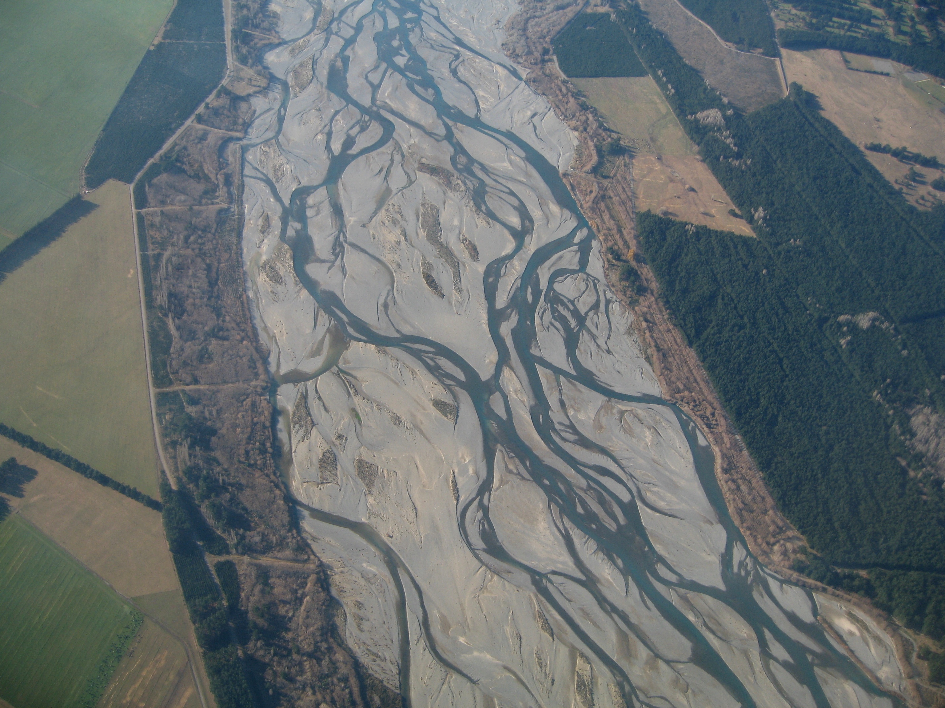
During the early Triassic (4–6 million years after the P–Tr extinction), the plant biomass was insufficient to form coal deposits, which implies a limited food mass for herbivores.^[14] River patterns in the Karoo changed from meandering to braided, indicating that vegetation there was very sparse for a long time.^[60]

Each major segment of the early Triassic ecosystem—plant and animal, marine and terrestrial—was dominated by a small number of genera, which appeared virtually worldwide, for example: the herbivorous therapsid Lystrosaurus (which accounted for about 90% of early Triassic land vertebrates) and the bivalves Claraia, Eumorphotis, Unionites and Promylina. A healthy ecosystem has a much larger number of genera, each living in a few preferred types of habitat.^[50][61]

Disaster taxa (opportunist organisms) took advantage of the devastated ecosystem and enjoyed a temporary population boom and increase in their territory. For example: Lingula (a brachiopod); stromatolites, which had been confined to marginal environments since the Ordovician; Pleuromeia (a small, weedy plant); Dicroidium (a seed fern).^{[11][61][62][63]}

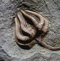Sessile filter feeders like this Crinoid were significantly less abundant after the P–Tr extinction.

Changes in marine ecosystems

Prior to the extinction, approximately 67% of marine animals were sessile and attached to the sea floor, but during the Mesozoic only about half of the marine animals were sessile while the rest were free living. Analysis of marine fossils from the period indicated a decrease in the abundance of sessile epifaunal suspension feeders, such as brachiopods and sea lilies, and an increase in more complex mobile species such as snails, urchins and crabs.^[64]

Before the Permian mass extinction event, both complex and simple marine ecosystems were equally common; after the recovery from the mass extinction, the complex communities outnumbered the simple communities by nearly three to one,^[64] and the increase in predation pressure led to the Mesozoic Marine Revolution.

Bivalves were fairly rare before the P–Tr extinction but became numerous and diverse in the Triassic and one group, the rudist clams, became the Mesozoic's main reef-builders. Some researchers think much of this change happened in the 5 million years between the two major extinction pulses.^[65]

Crinoids ("sea lilies") suffered a selective extinction, resulting in a decrease in the variety of their forms.^[66] Their ensuing adaptive radiation was brisk, and resulted in forms possessing flexible arms becoming widespread; motility, predominantly a response to predation pressure, also became far more prevalent.^[67]

Land vertebrates

Lystrosaurus was by far the most abundant early Triassic land vertebrate.

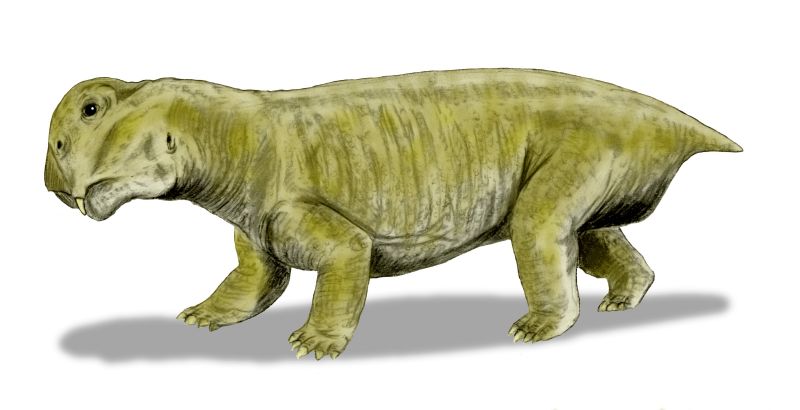
Lystrosaurus, a pig-sized herbivorous dicynodont therapsid, constituted as much as 90% of some earliest Triassic land vertebrate faunas.^[11] Smaller carnivorous cynodont therapsids also survived, including the ancestors of mammals. In the Karoo region of southern Africa the therocephalians Tetracynodon, Moschorhinus and Ictidosuchoides survived but do not appear to have been abundant in the Triassic.^[68]

Archosaurs (which included the ancestors of dinosaurs and crocodilians) were initially rarer than therapsids, but they began to displace therapsids in the mid-Triassic.^[11] In the mid to late Triassic the dinosaurs evolved from one group of archosaurs, and went on to dominate terrestrial ecosystems for the rest of the Mesozoic.^[69] This "Triassic Takeover" may have contributed to the evolution of mammals by forcing the surviving therapsids and their mammaliform successors to live as small, mainly nocturnal insectivores; nocturnal life probably forced at least the mammaliforms to develop fur and higher metabolic rates.^[70]

Some temnospondyl amphibians made a relatively quick recovery, in spite of nearly becoming extinct. Mastodonsaurus and trematosaurians were the main aquatic and semi-aquatic predators during most of the Triassic, some preying on tetrapods and others on fish.^[71]

Land vertebrates took an unusually long time to recover from the P–Tr extinction; writer M. J. Benton estimates that the recovery was not complete until 30 million years after the extinction, i.e. not until the Late Triassic, in which dinosaurs, pterosaurs, crocodiles, archosaurs, amphibians and mammaliforms were abundant and diverse.^[4]

Causes of the extinction event

Pin-pointing the exact cause (or causes) of the Permian-Triassic extinction event is a difficult undertaking, mostly due to the fact that the catastrophe occurred over 250 million years ago, and much of the evidence that would have pointed to the cause has either been destroyed by now or is concealed deep within the Earth under many layers of rock. The seafloor is also completely recycled every 200 million years due to the ongoing process of plate tectonics and seafloor spreading, thereby leaving no useful indications beneath the ocean. With the fairly significant evidence that scientists have managed to accumulate, there are several proposed mechanisms for the extinction event, including both catastrophic and gradualistic processes (similar to those theorized for the Cretaceous–Tertiary extinction event). The former include large or multiple bolide impact events, increased volcanism, or sudden release of methane hydrates from the sea floor. The latter include sea-level change, anoxia, and increasing aridity.^[11] Any hypothesis about the cause must explain the selectivity of the event, which primarily affected organisms with calcium carbonate skeletons; the long (4–6 million year) period before recovery started; and the minimal extent of biological mineralization (despite inorganic carbonates being deposited) once the recovery began.^[40]

Impact event

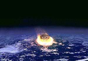Artist's impression of a major impact event. A collision between Earth and an asteroid a few kilometers in diameter would release as much energy as several million nuclear weapons detonating.

Evidence that an impact event may have caused the Cretaceous–Tertiary extinction event has led to speculation that similar impacts may have been the cause of other extinction events, including the P–Tr extinction, and therefore to a search for evidence of impacts at the times of other extinctions and for large impact craters of the appropriate age.

Reported evidence for an impact event from the P–Tr boundary level includes rare grains of shocked quartz in Australia and Antarctica;^[72][73] fullerenes trapping extraterrestrial noble gases;^[74] meteorite fragments in Antarctica;^[75] and grains rich in iron, nickel and silicon, which may have been created by an impact.^[76] However, the accuracy of most of these claims has been challenged.^{[77][78][79][80]} Quartz from Graphite Peak in Antarctica, for example, once considered "shocked," has recently been reexamined by optical and transmission electron microscopy. It was concluded that the observed features were not due to shock, but rather to plastic deformation, consistent with formation in a tectonic environment such as volcanism.^[81]

Several possible impact craters have been proposed as possible causes of the P–Tr extinction, including the Bedout structure off the northwest coast of Australia^[73] and the hypothesized Wilkes Land crater of East Antarctica.^[82][83] In each of these cases the idea that an impact was responsible has not been proven, and some have been widely criticized. In the case of Wilkes Land, the age of this sub-ice geophysical feature is very uncertain – it may be later than the Permian–Triassic extinction.

If impact is a major cause of the P–Tr extinction, it is likely that the crater would no longer exist. As 70% of the Earth's surface is sea, an asteroid or comet fragment is more than twice as likely to hit ocean as it is to hit land. However, Earth has no ocean-floor crust more than 200 million years old, because the "conveyor belt" process of sea-floor spreading and subduction destroys it within that time. It has also been speculated that craters produced by very large impacts may be masked by extensive flood basalting from below after the crust is punctured or weakened.^[84] Subduction should not, however, be entirely accepted as an explanation of why no firm evidence can be found: as with the K-T event, an ejecta blanket stratum rich in siderophilic elements (e.g., iridium) would be expected to be seen in formations from the time.

One attraction of large impact theories is that theoretically they could trigger other cause-considered extinction-paralleling phenomena,^[85] such as the Siberian Traps eruptions (see below) as being either an impact site^[86] or the antipode of an impact site.^[85][87] The abruptness of an impact also explains why species did not rapidly evolve in adaptation to more slowly-manifesting and/or less than global-in-scope phenomena.

Volcanism

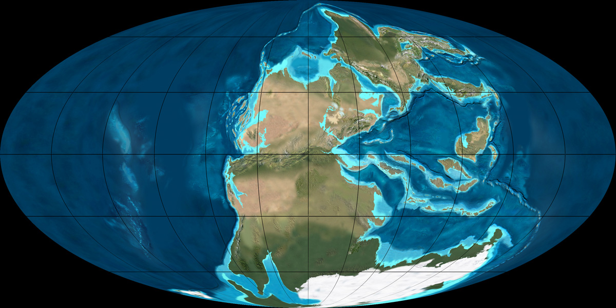
The world around the time of the P–Tr extinction. The Siberian Traps eruptions occurred on the eastern shore of the shallow sea (paler blue) at the north of the map. The earlier Emeishan eruptions occurred on the north edge of the almost enclosed shallow sea just north of the equator – at this time the blocks that currently form China and South-East Asia were just emerging.

The final stages of the Permian saw two flood basalt events. A small one, Emeishan Traps in China, occurred at the same time as the end-Guadalupian extinction pulse, in an area close to the equator at the time.^[88][89] The flood basalt eruptions that produced the Siberian Traps constituted one of the largest known volcanic events on Earth and covered over 2,000,000 square kilometres (770,000 sq mi) with lava.^[90][91][92] The Siberian Traps eruptions were formerly thought to have lasted for millions of years, but recent research dates them to 251.2 ± 0.3 Ma — immediately before the end of the Permian.^[2][93]

The Emeishan and Siberian Traps eruptions may have caused dust clouds and acid aerosols—which would have blocked out sunlight and thus disrupted photosynthesis both on land and in the photic zone of the ocean, causing food chains to collapse. These eruptions may also have caused acid rain when the aerosols washed out of the atmosphere. This may have killed land plants and molluscs and planktonic organisms which had calcium carbonate shells. The eruptions would also have emitted carbon dioxide, causing global warming. When all of the dust clouds and aerosols washed out of the atmosphere, the excess carbon dioxide would have remained and the warming would have proceeded without any mitigating effects.^[85]

The Siberian Traps had unusual features that made them even more dangerous. Pure flood basalts produce a lot of runny lava and do not hurl debris into the atmosphere. It appears, however, that 20% of the output of the Siberian Traps eruptions was pyroclastic, i.e. consisted of ash and other debris thrown high into the atmosphere, increasing the short-term cooling effect.^[94] The basalt lava erupted or intruded into carbonate rocks and into sediments that were in the process of forming large coal beds, both of which would have emitted large amounts of carbon dioxide, leading to stronger global warming after the dust and aerosols settled.^[85]

There is doubt, however, about whether these eruptions were enough on their own to cause a mass extinction as severe as the end-Permian. Equatorial eruptions are necessary to produce sufficient dust and aerosols to affect life worldwide, whereas the much larger Siberian Traps eruptions were inside or near the Arctic Circle. Furthermore, if the Siberian Traps eruptions occurred within a period of 200,000 years, the atmosphere's carbon dioxide content would have doubled. Recent climate models suggest that such a rise in CO₂ would have raised global temperatures by 1.5 °C (2.7 °F) to 4.5 °C (8.1 °F), which is unlikely to cause a catastrophe as great as the P–Tr extinction.^[85]

In January 2011, a team led by Stephen Grasby of the Geological Survey of Canada—Calgary, reported evidence that volcanism caused massive coal beds to ignite, possibly releasing more than 3 trillion tons of carbon. The team found ash deposits in deep rock layers near what is now Buchanan Lake. According to their article, "... coal ash dispersed by the explosive Siberian Trap eruption would be expected to have an associated release of toxic elements in impacted water bodies where fly ash slurries developed ...", and "Mafic megascale eruptions are long-lived events that would allow significant build-up of global ash clouds".^[95][96] In a statement, Grasby said "In addition to these volcanoes causing fires through coal, the ash it spewed was highly toxic and was released in the land and water, potentially contributing to the worst extinction event in earth history."^[97]

Methane hydrate gasification

Scientists have found worldwide evidence of a swift decrease of about 10% in the ¹³C/¹²C isotope ratio in carbonate rocks from the end-Permian.^[44][98] This is the first, largest and most rapid of a series of negative and positive excursions (decreases and increases in ¹³C/¹²C ratio) that continues until the isotope ratio abruptly stabilises in the middle Triassic, followed soon afterwards by the recovery of calcifying life forms (organisms that use calcium carbonate to build hard parts such as shells).^[12]

A variety of factors may have contributed to this drop in the ¹³C/¹²C ratio, but most turn out to be insufficient to account fully for it:^[99]

• Gases from volcanic eruptions have a ¹³C/¹²C ratio about 5 to 8 ‰ below standard (δ¹³C about −5 to −8 ‰). But the amount required to produce a reduction of about 10 ‰ worldwide requires eruptions greater by orders of magnitude than any for which evidence has been found.^[100]
• A reduction in organic activity would extract ¹²C more slowly from the environment and leave more of it to be incorporated into sediments, thus reducing the ¹³C/¹²C ratio. Biochemical processes use the lighter isotopes, since chemical reactions are ultimately driven by electromagnetic forces between atoms and lighter isotopes respond more quickly to these forces. But a study of a smaller drop of 3 to 4  ‰ in ¹³C/¹²C (δ¹³C −3 to −4 ‰) at the Paleocene-Eocene Thermal Maximum (PETM) concluded that even transferring all the organic carbon (in organisms, soils, and dissolved in the ocean) into sediments would be insufficient: even such a large burial of material rich in ¹²C would not have produced the smaller drop in the ¹³C/¹²C ratio of the rocks around the PETM.^[100]
• Buried sedimentary organic matter has a ¹³C/¹²C ratio 20 to 25 ‰ below normal (δ¹³C −20 to −25 ‰). Theoretically, if the sea level fell sharply, shallow marine sediments would be exposed to oxidization. But 6,500–8,400 gigatons (1 gigaton = 10⁹ metric tons) of organic carbon would have to be oxidized and returned to the ocean-atmosphere system within less than a few hundred thousand years to reduce the ¹³C/¹²C ratio by 10 ‰. This is not thought to be a realistic possibility.^[8]
• Rather than a sudden decline in sea level, intermittent periods of ocean-bottom hyperoxia and anoxia (high-oxygen and low- / zero-oxygen conditions) may have caused the ¹³C/¹²C ratio fluctuations in the Early Triassic;^[12] and global anoxia may have been responsible for the end-Permian blip. The continents of the end-Permian and early Triassic were more clustered in the tropics than they are now (see map above), and large tropical rivers would have dumped sediment into smaller, partially enclosed ocean basins in low latitudes. Such conditions favor oxic and anoxic episodes; oxic / anoxic conditions would result in a rapid release / burial respectively of large amounts of organic carbon, which has a low ¹³C/¹²C ratio because biochemical processes use the lighter isotopes.^[101] This, or another organic-based reason, may have been responsible for both this and a late Proterozoic/Cambrian pattern of fluctuating ¹³C/¹²C ratios.^[12]

Other hypotheses include mass oceanic poisoning releasing vast amounts of CO₂^[102] and a long-term reorganisation of the global carbon cycle.^[99]

However, only one sufficiently powerful cause has been proposed for the global 10 ‰ reduction in the ¹³C/¹²C ratio: the release of methane from methane clathrates;^[8] and carbon-cycle models confirm that it would have been sufficient to produce the observed reduction.^[99][102] Methane clathrates, also known as methane hydrates, consist of methane molecules trapped in cages of water molecules. The methane is produced by methanogens (microscopic single-celled organisms) and has a ¹³C/¹²C ratio about 60 ‰ below normal (δ¹³C −60  ‰). At the right combination of pressure and temperature it gets trapped in clathrates fairly close to the surface of permafrost and in much larger quantities at continental margins (continental shelves and the deeper seabed close to them). Oceanic methane hydrates are usually found buried in sediments where the seawater is at least 300 metres (980 ft) deep. They can be found up to about 2,000 metres (6,600 ft) below the sea floor, but usually only about 1,100 metres (3,600 ft) below the sea floor.^[103]

The area covered by lava from the Siberian Traps eruptions is about twice as large as was originally thought, and most of the additional area was shallow sea at the time. It is very likely that the seabed contained methane hydrate deposits and that the lava caused the deposits to dissociate, releasing vast quantities of methane.^[104]

One would expect a vast release of methane to cause significant global warming, since methane is a very powerful greenhouse gas. There is strong evidence that global temperatures increased by about 6 °C (10.8 °F) near the equator and therefore by more at higher latitudes: a sharp decrease in oxygen isotope ratios (¹⁸O/¹⁶O);^[105] the extinction of Glossopteris flora (Glossopteris and plants that grew in the same areas), which needed a cold climate, and its replacement by floras typical of lower paleolatitudes.^[11][106]

However, the pattern of isotope shifts expected to result from a massive release of methane do not match the patterns seen throughout the early Triassic. Not only would a methane cause require the release of five times as much methane as postulated for the PETM,^[12] but it would also have to be re-buried at an unrealistically high rate to account for the rapid increases in the ¹³C/¹²C ratio (episodes of high positive δ¹³C) throughout the early Triassic, before being released again several times.^[12]

Sea level fluctuations

Marine regression occurs when areas of submerged seafloor are exposed above sea level. This lowering of sea level causes a reduction in shallow marine habitats, leading to biotic turnover. Shallow marine habitats are productive areas for organisms at the bottom of the food chain, their loss increasing competition for food sources.^[107] There is some correlation between incidents of pronounced sea level regression and mass extinctions, but other evidence indicates there is no relationship and that regression may itself create new habitats.^[11] It has also been suggested that sea-level changes result in changes in sediment deposition rates and effects water temperature and salinity, resulting in a decline in marine diversity.^[108]

Anoxia

See also: Anoxic event

There is evidence that the oceans became anoxic (severely deficient in oxygen) towards the end of the Permian. There was a noticeable and rapid onset of anoxic deposition in marine sediments around East Greenland near the end of the Permian.^[109] The uranium/thorium ratios of several late Permian sediments indicate that the oceans were severely anoxic around the time of the extinction.^[110]

This would have been devastating for marine life, producing widespread die-offs except for anaerobic bacteria inhabiting the sea-bottom mud. There is also evidence that anoxic events can cause catastrophic hydrogen sulfide emissions from the sea floor (see below).

The sequence of events leading to anoxic oceans might have involved a period of global warming that reduced the temperature gradient between the equator and the poles, which slowed or even stopped the thermohaline circulation. The slow-down or stoppage of the thermohaline circulation could have reduced the mixing of oxygen in the ocean.^[110]

However, one research article suggests that the types of oceanic thermohaline circulation that may have existed at the end of the Permian are not likely to have supported deep-sea anoxia.^[111]

Hydrogen sulfide emissions

A severe anoxic event at the end of the Permian could have made sulfate-reducing bacteria the dominant force in oceanic ecosystems, causing vast emissions of hydrogen sulfide that poisoned plant and animal life on both land and sea, as well as severely weakening the ozone layer, exposing much of the life that remained to fatal levels of UV radiation.^[112] Indeed, anaerobic photosynthesis by Chlorobiaceae (green sulfur bacteria), and its accompanying hydrogen sulfide emissions, occurred from the end-Permian into the early Triassic. The fact that this anaerobic photosynthesis persisted into the early Triassic is consistent with fossil evidence that the recovery from the Permian–Triassic extinction was remarkably slow.^[113]

This theory has the advantage of explaining the mass extinction of plants, which ought otherwise to have thrived in an atmosphere with a high level of carbon dioxide. Fossil spores from the end-Permian further support the theory: many show deformities that could have been caused by ultraviolet radiation, which would have been more intense after hydrogen sulfide emissions weakened the ozone layer.

The supercontinent Pangaea

Map of Pangaea showing where today's continents were at the Permian–Triassic boundary

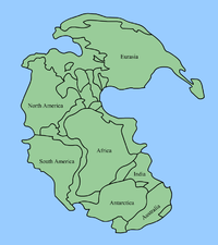
About half way through the Permian (in the Kungurian age of the Permian's Cisuralian epoch) all the continents joined to form the supercontinent Pangaea, surrounded by the superocean Panthalassa, although blocks that are now parts of Asia did not join the supercontinent until very late in the Permian.^[114] This configuration severely decreased the extent of shallow aquatic environments, the most productive part of the seas, and exposed formerly isolated organisms of the rich continental shelves to competition from invaders. Pangaea's formation would also have altered both oceanic circulation and atmospheric weather patterns, creating seasonal monsoons near the coasts and an arid climate in the vast continental interior.

Marine life suffered very high but not catastrophic rates of extinction after the formation of Pangaea (see the diagram "Marine genus biodiversity" at the top of this article)—almost as high as in some of the "Big Five" mass extinctions. The formation of Pangaea seems not to have caused a significant rise in extinction levels on land, and in fact most of the advance of the therapsids and increase in their diversity seems to have occurred in the late Permian, after Pangaea was almost complete. So it seems likely that Pangaea initiated a long period of increased marine extinctions but was not directly responsible for the "Great Dying" and the end of the Permian.

Combination of causes

Possible causes supported by strong evidence appear to describe a sequence of catastrophes, each one worse than the previous: the Siberian Traps eruptions were bad enough in their own right, but because they occurred near coal beds and the continental shelf, they also triggered very large releases of carbon dioxide and methane.^[56] The resultant global warming may have caused perhaps the most severe anoxic event in the oceans' history: according to this theory, the oceans became so anoxic that anaerobic sulfur-reducing organisms dominated the chemistry of the oceans and caused massive emissions of toxic hydrogen sulfide.^[56]

However, there may be some weak links in this chain of events: the changes in the ¹³C/¹²C ratio expected to result from a massive release of methane do not match the patterns seen throughout the early Triassic;^[12] and the types of oceanic thermohaline circulation, which may have existed at the end of the Permian are not likely to have supported deep-sea anoxia.^[111]

References

1. ^ "The Great Dying - NASA Science". http://science.nasa.gov/science-news/science-at-nasa/2002/28jan_extinction/. Retrieved 2011-04-30. 
2. ^ ^{a b c d e f g} Jin YG, Wang Y, Wang W, Shang QH, Cao CQ, Erwin DH (2000). "Pattern of Marine Mass Extinction Near the Permian–Triassic Boundary in South China". Science 289 (5478): 432–436. Bibcode 2000Sci...289..432J. doi:10.1126/science.289.5478.432. PMID 10903200. 
3. ^ ^{a b} Bowring SA, Erwin DH, Jin YG, Martin MW, Davidek K, Wang W (1998). "U/Pb Zircon Geochronology and Tempo of the End-Permian Mass Extinction". Science 280 (5366): 1039–1045. Bibcode 1998Sci...280.1039B. doi:10.1126/science.280.5366.1039. 
4. ^ ^{a b c} Benton M J (2005). When life nearly died: the greatest mass extinction of all time. London: Thames & Hudson. ISBN 0-500-28573-X. 
5. ^ ^{a b c d e} Sahney S and Benton M.J (2008). "Recovery from the most profound mass extinction of all time" (PDF). Proceedings of the Royal Society: Biological 275 (1636): 759–765. doi:10.1098/rspb.2007.1370. PMC 2596898. PMID 18198148. http://journals.royalsociety.org/content/qq5un1810k7605h5/fulltext.pdf. 
6. ^ ^{a b c} Labandeira CC, Sepkoski JJ (1993). "Insect diversity in the fossil record". Science 261 (5119): 310–315. Bibcode 1993Sci...261..310L. doi:10.1126/science.11536548. PMID 11536548. 
7. ^ Sole RV, Newman M (2003). "Extinctions and Biodiversity in the Fossil Record". In Canadell JG, Mooney, HA. Encyclopedia of Global Environmental Change, The Earth System - Biological and Ecological Dimensions of Global Environmental Change (Volume 2). New York: Wiley. pp. 297–391. ISBN 0-470-85361-1. 
8. ^ ^{a b c d e} Erwin DH (1993). The great Paleozoic crisis; Life and death in the Permian. Columbia University Press. ISBN 0231074670. 
9. ^ Yin H, Zhang K, Tong J, Yang Z, Wu S. The Global Stratotype Section and Point (GSSP) of the Permian-Triassic Boundary. 24. 102–114. 
10. ^ Yin HF, Sweets WC, Yang ZY, Dickins JM (1992). "Permo-Triassic events in the eastern Tethys–an overview". In Sweet WC. Permo-Triassic events in the eastern Tethys: stratigraphy, classification, and relations with the western Tethys. Cambridge, UK: Cambridge University Press. pp. 1–7. ISBN 0-521-54573-0. 
11. ^ ^{a b c d e f g} Tanner LH, Lucas SG & Chapman MG (2004). "Assessing the record and causes of Late Triassic extinctions" (PDF). Earth-Science Reviews 65 (1–2): 103–139. Bibcode 2004ESRv...65..103T. doi:10.1016/S0012-8252(03)00082-5. Archived from the original on 2007-10-25. http://web.archive.org/web/20071025225841/http://nmnaturalhistory.org/pdf_files/TJB.pdf. Retrieved 2007-10-22. 
12. ^ ^{a b c d e f g h i} Payne, J.L.; Lehrmann, D.J.; Wei, J.; Orchard, M.J.; Schrag, D.P.; Knoll, A.H. (2004). "Large Perturbations of the Carbon Cycle During Recovery from the End-Permian Extinction". Science 305 (5683): 506–9. doi:10.1126/science.1097023. PMID 15273391. http://www.sciencemag.org/cgi/content/abstract/305/5683/506. 
13. ^ ^{a b c d e f g h i j k l m} McElwain, J.C.; Punyasena, S.W. (2007). "Mass extinction events and the plant fossil record". Trends in Ecology & Evolution 22 (10): 548–557. doi:10.1016/j.tree.2007.09.003. PMID 17919771. 
14. ^ ^{a b c d e} Retallack, GJ; Veevers, JJ; Morante, R (1996). "Global coal gap between Permian–Triassic extinctions and middle Triassic recovery of peat forming plants". GSA Bulletin 108 (2): 195–207. doi:10.1130/0016-7606(1996)108<0195:GCGBPT>2.3.CO;2.  edit
15. ^ Erwin, D.H (1993). The Great Paleozoic Crisis: Life and Death in the Permian. New York: Columbia University Press. ISBN 0231074670. 
16. ^ Magaritz M (1989). "¹³C minima follow extinction events: a clue to faunal radiation". Geology 17 (4): 337–340. Bibcode 1989Geo....17..337M. doi:10.1130/0091-7613(1989)017<0337:CMFEEA>2.3.CO;2. 
17. ^ Krull SJ, Retallack JR (2000). "¹³C depth profiles from paleosols across the Permian–Triassic boundary: Evidence for methane release". GSA Bulletin 112 (9): 1459–1472. doi:10.1130/0016-7606(2000)112<1459:CDPFPA>2.0.CO;2. ISSN 0016-7606. 
18. ^ Dolenec T, Lojen S, Ramovs A (2001). "The Permian–Triassic boundary in Western Slovenia (Idrijca Valley section): magnetostratigraphy, stable isotopes, and elemental variations". Chemical Geology 175 (1): 175–190. doi:10.1016/S0009-2541(00)00368-5. 
19. ^ Musashi M, Isozaki Y, Koike T, Kreulen R (2001). "Stable carbon isotope signature in mid-Panthalassa shallow-water carbonates across the Permo–Triassic boundary: evidence for ¹³C-depleted ocean". Earth Planet. Sci. Lett. 193: 9–20. Bibcode 2001E&PSL.191....9M. doi:10.1016/S0012-821X(01)00398-3. 
20. ^ Dolenec T, Lojen S, Ramovs A (2001). "The Permian-Triassic boundary in Western Slovenia (Idrijca Valley section): magnetostratigraphy, stable isotopes, and elemental variations". Chemical Geology 175: 175–190. doi:10.1016/S0009-2541(00)00368-5. 
21. ^ Mauna Loa CO₂ annual mean data from NOAA. "Trend" data was used. See also: Trends in Carbon Dioxide from NOAA.
22. ^ ^{a b} H Visscher, H Brinkhuis, D L Dilcher, W C Elsik, Y Eshet, C V Looy, M R Rampino, and A Traverse (1996). "The terminal Paleozoic fungal event: Evidence of terrestrial ecosystem destabilization and collapse". Proceedings of the National Academy of Sciences 93 (5): 2155–2158. Bibcode 1996PNAS...93.2155V. doi:10.1073/pnas.93.5.2155. PMC 39926. PMID 11607638. http://www.pubmedcentral.nih.gov/articlerender.fcgi?tool=pmcentrez&artid=39926. 
23. ^ Foster, C.B.; Stephenson, M.H.; Marshall, C.; Logan, G.A.; Greenwood, P.F. (2002). "A Revision Of Reduviasporonites Wilson 1962: Description, Illustration, Comparison And Biological Affinities". Palynology 26 (1): 35–58. doi:10.2113/0260035. http://palynology.geoscienceworld.org/cgi/content/abstract/26/1/35. 
24. ^ López-Gómez, J. and Taylor, E.L. (2005). "Permian-Triassic Transition in Spain: A multidisciplinary approach". Palaeogeography, Palaeoclimatology, Palaeoecology 229 (1–2): 1–2. doi:10.1016/j.palaeo.2005.06.028. http://www.sciencedirect.com/science?_ob=ArticleURL&_udi=B6V6R-4GR8RWF-5&_user=1495569&_rdoc=1&_fmt=&_orig=search&_sort=d&view=c&_acct=C000053194&_version=1&_urlVersion=0&_userid=1495569&md5=537a1a5b0a8e04cca2221ecb12afb1e9. 
25. ^ Looy, C.V.; Twitchett, R.J.; Dilcher, D.L.; Van Konijnenburg-van Cittert, J.H.A.; Visscher, H. (2005). "Life in the end-Permian dead zone". Proceedings of the National Academy of Sciences 162 (4): 7879–7883. Bibcode 2001PNAS...98.7879L. doi:10.1073/pnas.131218098. PMC 35436. PMID 11427710. http://www.pubmedcentral.nih.gov/articlerender.fcgi?tool=pmcentrez&artid=35436. "See image 2" 
26. ^ ^{a b} Ward PD, Botha J, Buick R, De Kock MO, Erwin DH, Garrison GH, Kirschvink JL & Smith R (2005). "Abrupt and Gradual Extinction Among Late Permian Land Vertebrates in the Karoo Basin, South Africa". Science 307 (5710): 709–714. Bibcode 2005Sci...307..709W. doi:10.1126/science.1107068. PMID 15661973. 
27. ^ Retallack, G.J.; Smith, R.M.H.; Ward, P.D. (2003). "Vertebrate extinction across Permian-Triassic boundary in Karoo Basin, South Africa". Bulletin of the Geological Society of America 115 (9): 1133–1152. doi:10.1130/B25215.1. http://intl-bulletin.geoscienceworld.org/cgi/content/abstract/115/9/1133. 
28. ^ Sephton, Mark A.; Visscher, Henk; Looy, Cindy V.; Verchovsky, Alexander B.; Watson, Jonathon S. (2009). "Chemical constitution of a Permian-Triassic disaster species". Geology 37 (10): 875–878. doi:10.1130/G30096A.1. http://geology.gsapubs.org/content/37/10/875.abstract. 
29. ^ Rampino MR, Prokoph A & Adler A (2000). "Tempo of the end-Permian event: High-resolution cyclostratigraphy at the Permian–Triassic boundary". Geology 28 (7): 643–646. Bibcode 2000Geo....28..643R. doi:10.1130/0091-7613(2000)28<643:TOTEEH>2.0.CO;2. ISSN 0091-7613. 
30. ^ Wang, S.C.; Everson, P.J. (2007). "Confidence intervals for pulsed mass extinction events". Paleobiology 33 (2): 324–336. doi:10.1666/06056.1. 
31. ^ Twitchett RJ Looy CV Morante R Visscher H & Wignall PB (2001). "Rapid and synchronous collapse of marine and terrestrial ecosystems during the end-Permian biotic crisis". Geology 29 (4): 351–354. Bibcode 2001Geo....29..351T. doi:10.1130/0091-7613(2001)029<0351:RASCOM>2.0.CO;2. ISSN 0091-7613. 
32. ^ Retallack, G.J.; Metzger, C.A.; Greaver, T.; Jahren, A.H.; Smith, R.M.H.; Sheldon, N.D. (2006). "Middle-Late Permian mass extinction on land". Bulletin of the Geological Society of America 118 (11–12): 1398–1411. doi:10.1130/B26011.1. 
33. ^ Stanley SM & Yang X (1994). "A Double Mass Extinction at the End of the Paleozoic Era". Science 266 (5189): 1340–1344. Bibcode 1994Sci...266.1340S. doi:10.1126/science.266.5189.1340. PMID 17772839. 
34. ^ Retallack, G.J., Metzger, C.A., Jahren, A.H., Greaver, T., Smith, R.M.H., and Sheldon, N.D (November/December 2006). "Middle-Late Permian mass extinction on land". GSA Bulletin 118 (11/12): 1398–1411. doi:10.1130/B26011.1. 
35. ^ Ota, A, and Isozaki, Y. (March 2006). "Fusuline biotic turnover across the Guadalupian–Lopingian (Middle–Upper Permian) boundary in mid-oceanic carbonate buildups: Biostratigraphy of accreted limestone in Japan". Journal of Asian Earth Sciences 26 (3–4): 353–368. Bibcode 2006JAESc..26..353O. doi:10.1016/j.jseaes.2005.04.001. 
36. ^ Shen, S., and Shi, G.R. (2002). "Paleobiogeographical extinction patterns of Permian brachiopods in the Asian-western Pacific region". Paleobiology 28 (4): 449–463. doi:10.1666/0094-8373(2002)028<0449:PEPOPB>2.0.CO;2. ISSN 0094-8373. 
37. ^ Wang, X-D, and Sugiyama, T. (December 2000). "Diversity and extinction patterns of Permian coral faunas of China". Lethaia 33 (4): 285–294. doi:10.1080/002411600750053853. http://www.blackwell-synergy.com/doi/abs/10.1080/002411600750053853. 
38. ^ Racki G (1999). "Silica-secreting biota and mass extinctions: survival processes and patterns". Palaeogeography, Palaeoclimatology, Palaeoecology 154 (1–2): 107–132. doi:10.1016/S0031-0182(99)00089-9. 
39. ^ Bambach, R.K.; Knoll, A.H.; Wang, S.C. (December 2004). "Origination, extinction, and mass depletions of marine diversity". Paleobiology 30 (4): 522–542. doi:10.1666/0094-8373(2004)030<0522:OEAMDO>2.0.CO;2. ISSN 0094-8373. http://www.bioone.org.myaccess.library.utoronto.ca/perlserv/?request=get-document&issn=0094-8373&volume=30&page=522. 
40. ^ ^{a b} Knoll, A.H. ((2004)). "Biomineralization and evolutionary history. In: P.M. Dove, J.J. DeYoreo and S. Weiner (Eds), Reviews in Mineralogy and Geochemistry,". http://www.geochem.geos.vt.edu/bgep/pubs/Chapter_11_Knoll.pdf. 
41. ^ Stanley, S.M. (2008). "Predation defeats competition on the seafloor". Paleobiology 34 (1): 1–21. doi:10.1666/07026.1. http://paleobiol.geoscienceworld.org/cgi/content/short/34/1/1. Retrieved 2008-05-13. 
42. ^ Stanley, S.M. (2007). "An Analysis of the History of Marine Animal Diversity". Paleobiology 33 (sp6): 1–55. doi:10.1666/06020.1. http://paleobiol.geoscienceworld.org/cgi/content/abstract/33/4_Suppl/1. 
43. ^ McKinney, M.L. (1987). "Taxonomic selectivity and continuous variation in mass and background extinctions of marine taxa". Nature 325 (6100): 143–145. Bibcode 1987Natur.325..143M. doi:10.1038/325143a0. 
44. ^ ^{a b} Twitchett RJ, Looy CV, Morante R, Visscher H, Wignall PB (2001). "Rapid and synchronous collapse of marine and terrestrial ecosystems during the end-Permian biotic crisis". Geology 29 (4): 351–354. Bibcode 2001Geo....29..351T. doi:10.1130/0091-7613(2001)029<0351:RASCOM>2.0.CO;2. ISSN 0091-7613. 
45. ^ Knoll, A.H.; Bambach, R.K.; Canfield, D.E.; Grotzinger, J.P. (1996). "Comparative Earth history and Late Permian mass extinction". Science(Washington) 273 (5274): 452–457. Bibcode 1996Sci...273..452K. doi:10.1126/science.273.5274.452. PMID 8662528. 
46. ^ Leighton, L.R.; Schneider, C.L. (2008). "Taxon characteristics that promote survivorship through the Permian–Triassic interval: transition from the Paleozoic to the Mesozoic brachiopod fauna". Paleobiology 34 (1): 65–79. doi:10.1666/06082.1. 
47. ^ Villier, L.; Korn, D. (Oct 2004). "Morphological Disparity of Ammonoids and the Mark of Permian Mass Extinctions". Science 306 (5694): 264–266. Bibcode 2004Sci...306..264V. doi:10.1126/science.1102127. ISSN 0036-8075. PMID 15472073.  edit
48. ^ Saunders, W. B.; Greenfest-Allen, E.; Work, D. M.; Nikolaeva, S. V. (2008). "Morphologic and taxonomic history of Paleozoic ammonoids in time and morphospace". Paleobiology 34 (1): 128–154. doi:10.1666/07053.1.  edit
49. ^ Cascales-Miñana, B.; Cleal, C. J. (2011). "Plant fossil record and survival analyses". Lethaia: no–no. doi:10.1111/j.1502-3931.2011.00262.x.  edit
50. ^ ^{a b} Retallack, GJ (1995). "Permian–Triassic life crisis on land". Science 267 (5194): 77–80. Bibcode 1995Sci...267...77R. doi:10.1126/science.267.5194.77. PMID 17840061. 
51. ^ Looy, CV Brugman WA Dilcher DL & Visscher H (1999). "The delayed resurgence of equatorial forests after the Permian–Triassic ecologic crisis". Proceedings National Academy of Sciences 96 (24): 13857–13862. Bibcode 1999PNAS...9613857L. doi:10.1073/pnas.96.24.13857. PMC 24155. PMID 10570163. http://www.pubmedcentral.nih.gov/articlerender.fcgi?tool=pmcentrez&artid=24155. 
52. ^ Looy, CV; Twitchett RJ, Dilcher DL, &Van Konijnenburg-Van Cittert JHA and Henk Visscher. (July 3, 2001). "Life in the end-Permian dead zone". Proceedings of the National Academy of Sciences 14 (98): 7879–7883. doi:10.1073/pnas.131218098. PMC 35436. PMID 11427710. http://www.pubmedcentral.nih.gov/articlerender.fcgi?tool=pmcentrez&artid=35436. 
53. ^ Michaelsen P (2002). "Mass extinction of peat-forming plants and the effect on fluvial styles across the Permian–Triassic boundary, northern Bowen Basin, Australia". Palaeogeography, Palaeoclimatology, Palaeoecology 179 (3–4): 173–188. doi:10.1016/S0031-0182(01)00413-8. 
54. ^ Maxwell, W. D. (1992). "Permian and Early Triassic extinction of non-marine tetrapods". Palaeontology 35: 571–583. 
55. ^ Erwin DH (1990). "The End-Permian Mass Extinction". Annual Review of Ecology and Systematics 21: 69–91. doi:10.1146/annurev.es.21.110190.000441. 
56. ^ ^{a b c d e f} Knoll, A.H., Bambach, R.K., Payne, J.L., Pruss, S., and Fischer, W.W. (2007). "Paleophysiology and end-Permian mass extinction". Earth and Planetary Science Letters 256 (3–4): 295–313. Bibcode 2007E&PSL.256..295K. doi:10.1016/j.epsl.2007.02.018. http://pangea.stanford.edu/~jlpayne/Knoll%20et%20al%202007%20EPSL%20Permian%20Triassic%20paleophysiology.pdf. Retrieved 2008-07-04. 
57. ^ Claude E. Boyd (2000). Water quality: an introduction. Springer. pp. 121–. ISBN 9780792378532. http://books.google.com/books?id=aKgK83ANjk8C&pg=PA121. Retrieved 9 August 2010. 
58. ^ Payne, J.; Turchyn, A.; Paytan, A.; Depaolo, D.; Lehrmann, D.; Yu, M.; Wei, J. (2010). "Calcium isotope constraints on the end-Permian mass extinction". Proceedings of the National Academy of Sciences of the United States of America 107 (19): 8543–8548. Bibcode 2010PNAS..107.8543P. doi:10.1073/pnas.0914065107. PMC 2889361. PMID 20421502. http://www.pubmedcentral.nih.gov/articlerender.fcgi?tool=pmcentrez&artid=2889361.  edit
59. ^ Lehrmann, D.J., Ramezan, J., Bowring, S.A. et al. (December 2006). "Timing of recovery from the end-Permian extinction: Geochronologic and biostratigraphic constraints from south China". Geology 34 (12): 1053–1056. Bibcode 2006Geo....34.1053L. doi:10.1130/G22827A.1. http://geology.geoscienceworld.org/cgi/content/abstract/34/12/1053. 
60. ^ Ward PD, Montgomery DR, & Smith R (2000). "Altered river morphology in South Africa related to the Permian–Triassic extinction". Science 289 (5485): 1740–1743. Bibcode 2000Sci...289.1740W. doi:10.1126/science.289.5485.1740. PMID 10976065. 
61. ^ ^{a b} Hallam A & Wignall PB (1997). Mass Extinctions and their Aftermath. Oxford University Press. ISBN 978-0198549161. 
62. ^ Rodland, DL & Bottjer, DJ (2001). "Biotic Recovery from the End-Permian Mass Extinction: Behavior of the Inarticulate Brachiopod Lingula as a Disaster Taxon". PALAIOS 16 (1): 95–101. doi:10.1669/0883-1351(2001)016<0095:BRFTEP>2.0.CO;2. ISSN 0883-1351. 
63. ^ Zi-qiang W (1996). "Recovery of vegetation from the terminal Permian mass extinction in North China". Review of Palaeobotany and Palynology 91 (1–4): 121–142. doi:10.1016/0034-6667(95)00069-0. 
64. ^ ^{a b} Wagner PJ, Kosnik MA, & Lidgard S (2006). "Abundance Distributions Imply Elevated Complexity of Post-Paleozoic Marine Ecosystems". Science 314 (5803): 1289–1292. Bibcode 2006Sci...314.1289W. doi:10.1126/science.1133795. PMID 17124319. 
65. ^ Clapham, M.E., Bottjer, D.J. and Shen, S. (2006). "Decoupled diversity and ecology during the end-Guadalupian extinction (late Permian)". Geological Society of America Abstracts with Programs 38 (7): 117. http://gsa.confex.com/gsa/2006AM/finalprogram/abstract_111312.htm. Retrieved 2008-03-28. 
66. ^ Foote, M. (1999). "Morphological diversity in the evolutionary radiation of Paleozoic and post-Paleozoic crinoids" (PDF). Paleobiology 25 (sp1): 1–116. doi:10.1666/0094-8373(1999)25[1:MDITER]2.0.CO;2. ISSN 0094-8373. JSTOR 2666042.. 
67. ^ Baumiller, T. K. (2008). "Crinoid Ecological Morphology". Annual Review of Earth and Planetary Sciences 36 (1): 221–249. Bibcode 2008AREPS..36..221B. doi:10.1146/annurev.earth.36.031207.124116.  edit
68. ^ Botha, J., and Smith, R.M.H. (2007). "Lystrosaurus species composition across the Permo–Triassic boundary in the Karoo Basin of South Africa". Lethaia 40 (2): 125–137. doi:10.1111/j.1502-3931.2007.00011.x. http://www3.interscience.wiley.com/journal/117996985/abstract?CRETRY=1&SRETRY=0. Retrieved 2008-07-02.  Full version online at "Lystrosaurus species composition across the Permo–Triassic boundary in the Karoo Basin of South Africa" (PDF). http://www.nasmus.co.za/PALAEO/jbotha/pdfs/Botha%20and%20Smith%202007.pdf. Retrieved 2008-07-02. 
69. ^ Benton, M.J. (2004). Vertebrate Paleontology. Blackwell Publishers. xii–452. ISBN 0-632-05614-2. 
70. ^ Ruben, J.A., and Jones, T.D. (2000). "Selective Factors Associated with the Origin of Fur and Feathers". American Zoologist 40 (4): 585–596. doi:10.1093/icb/40.4.585. http://icb.oxfordjournals.org/cgi/content/full/40/4/585. 
71. ^ Yates AM & Warren AA (2000). "The phylogeny of the 'higher' temnospondyls (Vertebrata: Choanata) and its implications for the monophyly and origins of the Stereospondyli". Zoological Journal of the Linnean Society 128 (1): 77–121. doi:10.1111/j.1096-3642.2000.tb00650.x. Archived from the original on 2007-10-01. http://web.archive.org/web/20071001020940/http://www.ingentaconnect.com/content/ap/zj/2000/00000128/00000001/art00184;jsessionid=f6bl337idrkcp.alice?format=print. Retrieved 2008-01-18. 
72. ^ Retallack GJ, Seyedolali A, Krull ES, Holser WT, Ambers CP, Kyte FT (1998). "Search for evidence of impact at the Permian–Triassic boundary in Antarctica and Australia". Geology 26 (11): 979–982. Bibcode 1998Geo....26..979R. doi:10.1130/0091-7613(1998)026<0979:SFEOIA>2.3.CO;2. http://geology.geoscienceworld.org/cgi/content/abstract/26/11/979. 
    
73. ^ ^{a b} Becker L, Poreda RJ, Basu AR, Pope KO, Harrison TM, Nicholson C, Iasky R (2004). "Bedout: a possible end-Permian impact crater offshore of northwestern Australia". Science 304 (5676): 1469–1476. Bibcode 2004Sci...304.1469B. doi:10.1126/science.1093925. PMID 15143216. 
74. ^ Becker L, Poreda RJ, Hunt AG, Bunch TE, Rampino M (2001). "Impact event at the Permian–Triassic boundary: Evidence from extraterrestrial noble gases in fullerenes". Science 291 (5508): 1530–1533. Bibcode 2001Sci...291.1530B. doi:10.1126/science.1057243. PMID 11222855. 
75. ^ Basu AR, Petaev MI, Poreda RJ, Jacobsen SB, Becker L (2003). "Chondritic meteorite fragments associated with the Permian–Triassic boundary in Antarctica". Science 302 (5649): 1388–1392. Bibcode 2003Sci...302.1388B. doi:10.1126/science.1090852. PMID 14631038. 
76. ^ Kaiho K, Kajiwara Y, Nakano T, Miura Y, Kawahata H, Tazaki K, Ueshima M, Chen Z, Shi GR (2001). "End-Permian catastrophe by a bolide impact: Evidence of a gigantic release of sulfur from the mantle". Geology 29 (9): 815–818. Bibcode 2001Geo....29..815K. doi:10.1130/0091-7613(2001)029<0815:EPCBAB>2.0.CO;2. ISSN 0091-7613. http://geology.geoscienceworld.org/cgi/content/abstract/26/11/979. Retrieved 2007-10-22. 
77. ^ Farley KA, Mukhopadhyay S, Isozaki Y, Becker L, Poreda RJ (2001). "An extraterrestrial impact at the Permian–Triassic boundary?". Science 293 (5539): 2343a–2343. doi:10.1126/science.293.5539.2343a. PMID 11577203. 
78. ^ Koeberl C, Gilmour I, Reimold WU, Philippe Claeys P, Ivanov B (2002). "End-Permian catastrophe by bolide impact: Evidence of a gigantic release of sulfur from the mantle: Comment and Reply". Geology 30 (9): 855–856. Bibcode 2002Geo....30..855K. doi:10.1130/0091-7613(2002)030<0855:EPCBBI>2.0.CO;2. ISSN 0091-7613. 
79. ^ Isbell JL, Askin RA, Retallack GR (1999). "Search for evidence of impact at the Permian–Triassic boundary in Antarctica and Australia; discussion and reply". Geology 27 (9): 859–860. Bibcode 1999Geo....27..859I. doi:10.1130/0091-7613(1999)027<0859:SFEOIA>2.3.CO;2. 
80. ^ Koeberl K, Farley KA, Peucker-Ehrenbrink B, Sephton MA (2004). "Geochemistry of the end-Permian extinction event in Austria and Italy: No evidence for an extraterrestrial component". Geology 32 (12): 1053–1056. Bibcode 2004Geo....32.1053K. doi:10.1130/G20907.1. 
    
81. ^ Langenhorst F, Kyte FT & Retallack GJ (2005). "Reexamination of quartz grains from the Permian–Triassic boundary section at Graphite Peak, Antarctica" (PDF). Lunar and Planetary Science Conference XXXVI. http://www.lpi.usra.edu/meetings/lpsc2005/pdf/2358.pdf. Retrieved 2007-07-13. 
82. ^ von Frese RR, Potts L, Gaya-Pique L, Golynsky AV, Hernandez O, Kim J, Kim H & Hwang J (2006). Abstract "Permian–Triassic mascon in Antarctica". Eos Trans. AGU, Jt. Assem. Suppl. 87 (36): Abstract T41A–08. http://www.agu.org/cgi-bin/SFgate/SFgate?language=English&verbose=0&listenv=table&application=sm06&convert=&converthl=&refinequery=&formintern=&formextern=&transquery=von%20frese&_lines=&multiple=0&descriptor=%2fdata%2fepubs%2fwais%2findexes%2fsm06%2fsm06%7c789%7c3849%7cPermian-Triassic%20Mascon%20in%20Antarctica%7cHTML%7clocalhost:0%7c%2fdata%2fepubs%2fwais%2findexes%2fsm06%2fsm06%7c6292543%206296392%20%2fdata2%2fepubs%2fwais%2fdata%2fsm06%2fsm06.txt Abstract. Retrieved 2007-10-22. 
83. ^ Von Frese, R.R.B.; L. V. Potts, S. B. Wells, T. E. Leftwich, H. R. Kim, J. W. Kim, A. V. Golynsky, O. Hernandez, and L. R. Gaya-Piqué (2009). "GRACE gravity evidence for an impact basin in Wilkes Land, Antarctica". Geochem. Geophys. Geosyst. 10 (2): Q02014. Bibcode 2009GGG....1002014V. doi:10.1029/2008GC002149. 
84. ^ Jones AP, Price GD, Price NJ, DeCarli PS, Clegg RA (2002). "Impact induced melting and the development of large igneous provinces". Earth and Planetary Science Letters 202 (3): 551–561. Bibcode 2002E&PSL.202..551J. doi:10.1016/S0012-821X(02)00824-5. 
85. ^ ^{a b c d e} White RV (2002). "Earth's biggest 'whodunnit': unravelling the clues in the case of the end-Permian mass extinction" (PDF). Phil. Trans. Royal Society of London 360 (1801): 2963–2985. Bibcode 2002RSPTA.360.2963W. doi:10.1098/rsta.2002.1097. PMID 12626276. http://www.le.ac.uk/gl/ads/SiberianTraps/Documents/White2002-P-Tr-whodunit.pdf. Retrieved 2008-01-12. 
86. ^ AHager, Bradford H (2001). "Giant Impact Craters Lead To Flood Basalts: A Viable Model". CCNet 33/2001: Abstract 50470. http://abob.libs.uga.edu/bobk/ccc/cc030101.html. 
87. ^ Hagstrum, Jonathan T (2001). "Large Oceanic Impacts As The Cause Of Antipodal Hotspots And Global Mass Extinctions". CCNet 33/2001: Abstract 50288. http://abob.libs.uga.edu/bobk/ccc/cc030101.html. 
88. ^ Zhou, M-F., Malpas, J, Song, X-Y, Robinson, PT, Sun, M, Kennedy, AK, Lesher, CM & Keays, RR (2002). "A temporal link between the Emeishan large igneous province (SW China) and the end-Guadalupian mass extinction". Earth and Planetary Science Letters 196 (3–4): 113–122. Bibcode 2002E&PSL.196..113Z. doi:10.1016/S0012-821X(01)00608-2. 
89. ^ Wignall, Paul B. et al. (2009). "Volcanism, Mass Extinction, and Carbon Isotope Fluctuations in the Middle Permian of China". Science 324 (5931): 1179–1182. Bibcode 2009Sci...324.1179W. doi:10.1126/science.1171956. PMID 19478179. 
90. ^ Andy Saunders, Marc Reichow (2009). "The Siberian Traps - Area and Volume". http://www.le.ac.uk/gl/ads/SiberianTraps/AreaVolume.html. Retrieved 2009-10-18. 
91. ^ Andy Saunders and Marc Reichow (January 2009). "The Siberian Traps and the End-Permian mass extinction: a critical review". Chinese Science Bulletin (Springer) 54 (1): 20–37. doi:10.1007/s11434-008-0543-7. http://www.le.ac.uk/gl/ads/SiberianTraps/PDF%20Files/The%20Siberian%20Traps%20and%20the%20End-Permian%20mass.pdf. Retrieved 09-04-2010 
92. ^ Reichow, Marc K.; M.S. Pringle, A.I. Al'Mukhamedov, M.B. Allen, V.L. Andreichev, M.M. Buslov, C.E. Davies, G.S. Fedoseev, J.G. Fitton, S. Inger, A.Ya. Medvedev, C. Mitchell, V.N. Puchkov, I.Yu. Safonova, R.A. Scott, A.D. Saunders (2009). "The timing and extent of the eruption of the Siberian Traps large igneous province: Implications for the end-Permian environmental crisis". Earth and Planetary Science Letters 277: 9–20. Bibcode 2009E&PSL.277....9R. doi:10.1016/j.epsl.2008.09.030. http://www.le.ac.uk/gl/ads/SiberianTraps/PDF%20Files/Reichow%20et%20al.%202009.pdf. Retrieved 09-04-2010. 
93. ^ Mundil, R., Ludwig, K.R., Metcalfe, I. & Renne, P.R (2004). "Age and Timing of the Permian Mass Extinctions: U/Pb Dating of Closed-System Zircons". Science 305 (5691): 1760–1763. Bibcode 2004Sci...305.1760M. doi:10.1126/science.1101012. PMID 15375264. 
94. ^ "Permian–Triassic Extinction - Volcanism"
95. ^ Dan Verango (January 24, 2011). "Ancient mass extinction tied to torched coal". USA Today. http://content.usatoday.com/communities/sciencefair/post/2011/01/ancient-mass-extinction-tied-to-torched-coal-/1. 
96. ^ Stephen E. Grasby, Hamed Sanei & Benoit Beauchamp (January 23, 2011). "Catastrophic dispersion of coal fly ash into oceans during the latest Permian extinction". Nature Geoscience 4 (2): 104–107. Bibcode 2011NatGe...4..104G. doi:10.1038/ngeo1069. http://www.nature.com/ngeo/journal/vaop/ncurrent/full/ngeo1069.html. 
97. ^ "Researchers find smoking gun of world's biggest extinction; Massive volcanic eruption, burning coal and accelerated greenhouse gas choked out life". University of Calgary. January 23, 2011. http://www.eurekalert.org/pub_releases/2011-01/uoc-rfs012111.php. Retrieved 2011-01-26. 
98. ^ Palfy J, Demeny A, Haas J, Htenyi M, Orchard MJ, & Veto I (2001). "Carbon isotope anomaly at the Triassic– Jurassic boundary from a marine section in Hungary". Geology 29 (11): 1047–1050. Bibcode 2001Geo....29.1047P. doi:10.1130/0091-7613(2001)029<1047:CIAAOG>2.0.CO;2. ISSN 0091-7613. 
99. ^ ^{a b c} Berner, R.A. (2002). "Examination of hypotheses for the Permo-Triassic boundary extinction by carbon cycle modeling". Proceedings of the National Academy of Sciences 99 (7): 4172–4177. Bibcode 2002PNAS...99.4172B. doi:10.1073/pnas.032095199. PMC 123621. PMID 11917102. http://www.pubmedcentral.nih.gov/articlerender.fcgi?tool=pmcentrez&artid=123621. 
100. ^ ^{a b} Dickens GR, O'Neil JR, Rea DK & Owen RM (1995). "Dissociation of oceanic methane hydrate as a cause of the carbon isotope excursion at the end of the Paleocene". Paleoceanography 10 (6): 965–71. Bibcode 1995PalOc..10..965D. doi:10.1029/95PA02087. 
101. ^ Schrag, D.P., Berner, R.A., Hoffman, P.F., and Halverson, G.P. (2002). "On the initiation of a snowball Earth". Geochemistry Geophysics Geosystems 3 (6): 1036. doi:10.1029/2001GC000219. http://www.agu.org/pubs/crossref/2002/2001GC000219.shtml.  Preliminary abstract at Schrag, D.P. (June 2001). "On the initiation of a snowball Earth". Geological Society of America. http://gsa.confex.com/gsa/2001ESP/finalprogram/abstract_8038.htm. 
102. ^ ^{a b} Benton, M.J.; Twitchett, R.J. (2003). "How to kill (almost) all life: the end-Permian extinction event". Trends in Ecology & Evolution 18 (7): 358–365. doi:10.1016/S0169-5347(03)00093-4. 
103. ^ Dickens GR (2001). "The potential volume of oceanic methane hydrates with variable external conditions". Organic Geochemistry 32 (10): 1179–1193. doi:10.1016/S0146-6380(01)00086-9. 
104. ^ Reichow MK, Saunders AD, White RV, Pringle MS, Al'Muhkhamedov AI, Medvedev AI & Kirda NP (2002). "⁴⁰Ar/³⁹Ar Dates from the West Siberian Basin: Siberian Flood Basalt Province Doubled". Science 296 (5574): 1846–1849. Bibcode 2002Sci...296.1846R. doi:10.1126/science.1071671. PMID 12052954. 
105. ^ Holser WT, Schoenlaub H-P, Attrep Jr M, Boeckelmann K, Klein P, Magaritz M, Orth CJ, Fenninger A, Jenny C, Kralik M, Mauritsch H, Pak E, Schramm J-F, Stattegger K & Schmoeller R (1989). "A unique geochemical record at the Permian/Triassic boundary". Nature 337 (6202): 39–44. Bibcode 1989Natur.337...39H. doi:10.1038/337039a0. 
106. ^ Dobruskina IA (1987). "Phytogeography of Eurasia during the early Triassic". Palaeogeography, Palaeoclimatology, Palaeoecology 58 (1–2): 75–86. doi:10.1016/0031-0182(87)90007-1. 
107. ^ Newell ND (1971). "An Outline History of Tropical Organic Reefs" (PDF). American Museum novitates 2465: 1–37. http://digitallibrary.amnh.org/dspace/bitstream/2246/2673/1/N2465.pdf. Retrieved 2007-11-03. 
108. ^ McRoberts, C.A., Furrer, H., Jones, D.S. (1997). "Palaeoenvironmental interpretation of a Triassic– Jurassic boundary section from western Austria based on palaeoecological and geochemical data". Palaeogeography Palaeoclimatology Palaeoecology 136 (1–4): 79–95. doi:10.1016/S0031-0182(97)00074-6. 
109. ^ Wignall PB & Twitchett RJ (2002). "Permian–Triassic sedimentology of Jameson Land, East Greenland: Incised submarine channels in an anoxic basin". Journal of the Geological Society 159 (6): 691–703. doi:10.1144/0016-764900-120. 
110. ^ ^{a b} Monastersky, R. (May 25, 1996). "Oxygen starvation decimated Permian oceans". Science News. http://findarticles.com/p/articles/mi_m1200/is_n21_v149/ai_18351222. 
111. ^ ^{a b} Zhang R, Follows, MJ, Grotzinger, JP, & Marshall J (2001). "Could the Late Permian deep ocean have been anoxic?". Paleoceanography 16 (3): 317–329. Bibcode 2001PalOc..16..317Z. doi:10.1029/2000PA000522. http://www.agu.org/pubs/crossref/2001/2000PA000522.shtml. 
112. ^ Kump LR, Pavlov A, & Arthur MA (2005). "Massive release of hydrogen sulfide to the surface ocean and atmosphere during intervals of oceanic anoxia". Geology 33 (5): 397–400. Bibcode 2005Geo....33..397K. doi:10.1130/G21295.1. 
113. ^ Grice K, Cao C, Love GD, Bottcher ME, Twitchett RJ, Grosjean E, Summons RE, Turgeon SC, Dunning W & Yugan J (2005). "Photic Zone Euxinia During the Permian–Triassic Superanoxic Event". Science 307 (5710): 706–709. Bibcode 2005Sci...307..706G. doi:10.1126/science.1104323. PMID 15661975. 
114. ^ The Permian - Palaeos

Further reading

• Over, Jess (editor), Understanding Late Devonian and Permian–Triassic Biotic and Climatic Events, (Volume 20 in series Developments in Palaeontology and Stratigraphy (2006). The state of the inquiry into the extinction events.
• Sweet, Walter C. (editor), Permo–Triassic Events in the Eastern Tethys : Stratigraphy Classification and Relations with the Western Tethys (in series World and Regional Geology)

External links

• "Siberian Traps". http://www.le.ac.uk/gl/ads/SiberianTraps/Index.html. Retrieved 2011-04-30. 
• "Big Bang In Antarctica: Killer Crater Found Under Ice". http://www.sciencedaily.com/releases/2006/06/060601174729.htm. Retrieved 2011-04-30. 
• "Global Warming Led To Atmospheric Hydrogen Sulfide And Permian Extinction". http://www.sciencedaily.com/releases/2005/02/050223130549.htm. Retrieved 2011-04-30. 
• Morrison D. "Did an Impact Trigger the Permian-Triassic Extinction?". NASA. http://nai.arc.nasa.gov/news_stories/news_detail.cfm?ID=286. Retrieved 2011-04-30. 
• "Permian Extinction Event". http://www.historyfiles.co.uk/FeaturesPrehistory/Permian_Extinction01.htm. Retrieved 2011-04-30. 

Extinction eventsv · d · e

Minor events

↓End-Ediacaran?

↓Lau event

↓Toarcian turnover

↓Aptian

↓Cenomanian-Turonian

↓Middle Miocene
    disruption

↓Cambro-Ordovician

↓Ordo-Silurian

↓Late Devonian

↓Permo-Triassic

↓Triassic–Jurassic

↓Cretaceous-Tertiary

Major events

 

Ediacaran

 

 

Cambrian

 

 

Ordovician

 

 

Silurian

 

 

Devonian

 

 

Carboniferous

 

 

Permian

 

 

Triassic

 

 

Jurassic

 

 

Cretaceous

 

 

Palæogene

 

 

Neo-
gene

 

 

Neoproterozoic

 

 

Palæozoic

 

 

Mesozoic

 

 

Cenozoic

 

 

|

-600

|

-550

|

-500

|

-450

|

-400

|

-350

|

-300

|

-250

|

-200

|

-150

|

-100

|

-50

|

0

Millions of years before present