Dirichlet distribution

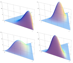Several images of the probability density of the Dirichlet distribution when K=3 for various parameter vectors α. Clockwise from top left: α=(6, 2, 2), (3, 7, 5), (6, 2, 6), (2, 3, 4).

In probability and statistics, the Dirichlet distribution (after Johann Peter Gustav Lejeune Dirichlet), often denoted $\operatorname{Dir}(\boldsymbol\alpha)$, is a family of continuous multivariate probability distributions parametrized by a vector $\boldsymbol\alpha$ of positive reals. It is the multivariate generalization of the beta distribution. Dirichlet distributions are very often used as prior distributions in Bayesian statistics, and in fact the Dirichlet distribution is the conjugate prior of the categorical distribution and multinomial distribution. That is, its probability density function returns the belief that the probabilities of K rival events are x_i given that each event has been observed α_i − 1 times.

The infinite-dimensional generalization of the Dirichlet distribution is the Dirichlet process.

Probability density function

Illustrating how the log of the density function changes when K=3 as we change the vector α from α=(0.3, 0.3, 0.3) to (2.0, 2.0, 2.0), keeping all the individual α_i's equal to each other.

The Dirichlet distribution of order K ≥ 2 with parameters α₁, ..., α_K > 0 has a probability density function with respect to Lebesgue measure on the Euclidean space R^K–1 given by

$f(x_1,\dots, x_{K-1}; \alpha_1,\dots, \alpha_K) = \frac{1}{\mathrm{B}(\alpha)} \prod_{i=1}^K x_i^{\alpha_i - 1}$

for all x₁, ..., x_K–1 > 0 satisfying x₁ + ... + x_K–1 < 1, where x_K is an abbreviation for 1 – x₁ – ... – x_K–1. The density is zero outside this open (K − 1)-dimensional simplex.

The normalizing constant is the multinomial beta function, which can be expressed in terms of the gamma function:

$\mathrm{B}(\alpha) = \frac{\prod_{i=1}^K \Gamma(\alpha_i)}{\Gamma\bigl(\sum_{i=1}^K \alpha_i\bigr)},\qquad\alpha=(\alpha_1,\dots,\alpha_K).$

Support

The support of the Dirichlet distribution is the set of K-dimensional vectors $\boldsymbol x$ whose entries are real numbers in the interval (0,1); furthermore, $||\boldsymbol x||_1=1$, i.e. the sum of the coordinates is 1. These can be viewed as the probabilities of a K-way categorical event. Another way to express this is that the domain of the Dirichlet distribution is itself a probability distribution, specifically a K-dimensional discrete distribution. Note that the technical term for the set of points in the support of a K-dimensional Dirichlet distribution is the open standard K − 1-simplex, which is a generalization of a triangle, embedded in the next-higher dimension. For example, with K = 3, the support looks like an equilateral triangle embedded in a downward-angle fashion in three-dimensional space, with vertices at (1,0,0),(0,1,0) and (0,0,1), i.e. touching each of the coordinate axes at a point 1 unit away from the origin.

A very common special case is the symmetric Dirichlet distribution, where all of the elements making up the parameter vector $\boldsymbol\alpha$ have the same value. Symmetric Dirichlet distributions are often used when a Dirichlet prior is called for, since there typically is no prior knowledge favoring one component over another. Since all elements of the parameter vector have the same value, the distribution alternatively can be parametrized by a single scalar value α, called the concentration parameter. When this value is 1, the symmetric Dirichlet distribution is equivalent to a uniform distribution over the open standard standard K − 1-simplex, i.e. it is uniform over all points in its support. Values of the concentration parameter above 1 prefer variates that are dense, evenly-distributed distributions, i.e. all probabilities returned are similar to each other. Values of the concentration parameter below 1 prefer sparse distributions, i.e. most of the probabilities returned will be close to 0, and the vast majority of the mass will be concentrated in a few of the probabilities.

Properties

Moments

Let $X = (X_1, \ldots, X_K)\sim\operatorname{Dir}(\alpha)$, meaning that the first K – 1 components have the above density and

$X_K=1-X_1-\cdots-X_{K-1}.$

Define $\textstyle\alpha_0 = \sum_{i=1}^K\alpha_i$. Then^[1]

$\mathrm{E}[X_i] = \frac{\alpha_i}{\alpha_0},$

$\mathrm{Var}[X_i] = \frac{\alpha_i (\alpha_0-\alpha_i)}{\alpha_0^2 (\alpha_0+1)}.$

Furthermore, if $i\neq j$

$\mathrm{Cov}[X_i,X_j] = \frac{- \alpha_i \alpha_j}{\alpha_0^2 (\alpha_0+1)}.$

(Note that the matrix so defined is singular.).

Mode

The mode of the distribution is^{[citation needed]} the vector (x₁, ..., x_K) with

$x_i = \frac{\alpha_i - 1}{\alpha_0 - K}, \quad \alpha_i > 1.$

Marginal distributions

The marginal distributions are Beta distributions^[2]:

$X_i \sim \operatorname{Beta}(\alpha_i, \alpha_0 - \alpha_i).$

Conjugate to multinomial

The Dirichlet distribution is conjugate to the multinomial distribution in the following sense: if

$\beta \mid X=(\beta_1, \ldots, \beta_{K}) \sim \operatorname{Mult}(X),$

where β_i is the number of occurrences of i in a sample of n points from the discrete distribution on {1, ..., K} defined by X, then^{[citation needed]}

$X \mid \beta \sim \operatorname{Dir}(\alpha + \beta).$

This relationship is used in Bayesian statistics to estimate the hidden parameters, X, of a categorical distribution (discrete probability distribution) given a collection of n samples. Intuitively, if the prior is represented as Dir(α), then Dir(α + β) is the posterior following a sequence of observations with histogram β.

Entropy

If X is a Dir(α) random variable, then the exponential family differential identities can be used to get an analytic expression for the expectation of log(X_i) and its associated covariance matrix:^{[citation needed]}

$\operatorname{E}[\log(X_i)] = \psi(\alpha_i)-\psi(\alpha_0)$

and

$\operatorname{Cov}[\log(X_i),\log(X_j)] = \psi'(\alpha_i) \delta_{ij} - \psi'(\alpha_0)$

where ψ is the digamma function, ψ' is the trigamma function, and δ_ij is the Kronecker delta. The formula for $\operatorname{E}[\log(X_i)]$ yields the following formula for the information entropy of X:^{[citation needed]}

$H(X) = \log \mathrm{B}(\alpha) + (\alpha_0-K)\psi(\alpha_0) - \sum_{j=1}^K (\alpha_j-1)\psi(\alpha_j)$

Aggregation

If $X = (X_1, \ldots, X_K)\sim\operatorname{Dir}(\alpha_1,\ldots,\alpha_K)$ then, if the random variables with subscripts i and j are dropped from the vector and replaced by their sum,

$X' = (X_1, \ldots, X_i + X_j, \ldots, X_K)\sim\operatorname{Dir}(\alpha_1,\ldots,\alpha_i+\alpha_j,\ldots,\alpha_K).$

This aggregation property may be used to derive the marginal distribution of X_i mentioned above.

Neutrality

Main article: Neutral vector

If $X = (X_1, \ldots, X_K)\sim\operatorname{Dir}(\alpha)$, then the vector X is said to be neutral^[3] in the sense that X_K is independent of X^{( − K)[citation needed]} where

$X^{(-K)}=(\frac{X_1}{1-X_K},\frac{X_2}{1-X_K},\ldots,\frac{X_{K-1}}{1-X_K}),$

and similarly for removing any of $X_2,\ldots,X_{K-1}$. Observe that any permutation of X is also neutral (a property not possessed by samples drawn from a generalized Dirichlet distribution^{[citation needed]}).

Related distributions

If, for $i\in\{1,2,\ldots,K\},$

$Y_i\sim\operatorname{Gamma}(\textrm{shape}=\alpha_i,\textrm{scale}=\theta)\text{ independently},$

then^{[citation needed]}

$V=\sum_{i=1}^K Y_i\sim\operatorname{Gamma}(\textrm{shape}=\sum_{i=1}^K\alpha_i,\textrm{scale}=\theta),$

and

$X = (X_1,\ldots,X_K) = (Y_1/V,\ldots,Y_K/V)\sim \operatorname{Dir}(\alpha_1,\ldots,\alpha_K).$

Although the X_is are not independent from one another, they can be seen to be generated from a set of K independent gamma random variables (see ^[4] for proof) . Unfortunately, since the sum V is lost in forming X, it is not possible to recover the original gamma random variables from these values alone. Nevertheless, because independent random variables are simpler to work with, this reparametrization can still be useful for proofs about properties of the Dirichlet distribution.

Applications

Multinomial opinions^{[clarification needed]} in subjective logic are equivalent to Dirichlet distributions.

Random number generation

Gamma distribution

A fast method to sample a random vector $x=(x_1, \ldots, x_K)$ from the K-dimensional Dirichlet distribution with parameters $(\alpha_1, \ldots, \alpha_K)$ follows immediately from this connection. First, draw K independent random samples $y_1, \ldots, y_K$ from gamma distributions each with density

$\textrm{Gamma}(\alpha_i, 1) = \frac{y_i^{\alpha_i-1} \; e^{-y_i}}{\Gamma (\alpha_i)}, \!$

and then set

$x_i = y_i/\sum_{j=1}^K y_j. \!$

Below is example python code to draw the sample:

params = [a1, a2, ..., ak]
sample = [random.gammavariate(a,1) for a in params]
sample = [v/sum(sample) for v in sample]

Marginal beta distributions

A less efficient algorithm^[5] relies on the univariate marginal and conditional distributions being beta and proceeds as follows. Simulate x₁ from a $\textrm{Beta}(\alpha_1, \sum_{i=2}^K \alpha_i)$ distribution. Then simulate $x_2, \ldots, x_{K-1}$ in order, as follows. For $j=2, \ldots, K-1$, simulate ϕ_j from a $\textrm{Beta}(\alpha_j, \sum_{i=j+1}^K \alpha_i)$ distribution, and let $x_j=(1-\sum_{i=1}^{j-1} x_i)\phi_j$. Finally, set $x_K=1-\sum_{i=1}^{K-1} x_i$.

Below is example python code to draw the sample:

params = [a1, a2, ..., ak]
xs = [random.betavariate(params[0], sum(params[1:]))]
for j in range(1,len(params)-1):
    phi = random.betavariate(params[j], sum(params[j+1:]))
    xs.append((1-sum(xs)) * phi)
xs.append(1-sum(xs))

Intuitive interpretations of the parameters

The concentration parameter

Dirichlet distributions are very often used as prior distributions in Bayesian inference. The simplest and perhaps most common type of Dirichlet prior is the symmetric Dirichlet distribution, where all parameters are equal. This corresponds to the case where you have no prior information to favor one component over any other. As described above, the single value α to which all parameters are set is called the concentration parameter. If the sample space of the Dirichlet distribution is interpreted as a discrete probability distribution, then intuitively the concentration parameter can be thought of as determining how "concentrated" the probability mass of a sample from a Dirichlet distribution is likely to be. With a value much less than 1, the mass will be highly concentrated in a few components, and all the rest will have almost no mass. With a value much greater than 1, the mass will be dispersed almost equally among all the components. See the article on the concentration parameter for further discussion.

String cutting

One example use of the Dirichlet distribution is if one wanted to cut strings (each of initial length 1.0) into K pieces with different lengths, where each piece had a designated average length, but allowing some variation in the relative sizes of the pieces. The α/α₀ values specify the mean lengths of the cut pieces of string resulting from the distribution. The variance around this mean varies inversely with α₀.

Pólya's urn

Consider an urn containing balls of K different colors. Initially, the urn contains α₁ balls of color 1, α₂ balls of color 2, and so on. Now perform N draws from the urn, where after each draw, the ball is placed back into the urn with an additional ball of the same color. In the limit as N approaches infinity, the proportions of different colored balls in the urn will be distributed as Dir(α₁,...,α_K).^[6]

For a formal proof, note that the proportions of the different colored balls form a bounded [0,1]^K-valued martingale, hence by the martingale convergence theorem, these proportions converge almost surely and in mean to a limiting random vector. To see that this limiting vector has the above Dirichlet distribution, check that all mixed moments agree.

Note that each draw from the urn modifies the probability of drawing a ball of any one color from the urn in the future. This modification diminishes with the number of draws, since the relative effect of adding a new ball to the urn diminishes as the urn accumulates increasing numbers of balls. This "diminishing returns" effect can also help explain how large α values yield Dirichlet distributions with most of the probability mass concentrated around a single point on the simplex.

See also

• Beta distribution
• Binomial distribution
• Categorical distribution
• Generalized Dirichlet distribution
• Latent Dirichlet allocation
• Dirichlet process
• Multinomial distribution
• Multivariate Pólya distribution

References

1. ^ Eq. (49.9) on page 488 of Kotz, Balakrishnan & Johnson (2000). Continuous Multivariate Distributions. Volume 1: Models and Applications. New York: Wiley.
2. ^ Ferguson, Thomas S. (1973). "A Bayesian analysis of some nonparametric problems". The Annals of Statistics 1 (2): 209–230. doi:10.1214/aos/1176342360. 
3. ^ Connor, Robert J.; Mosimann, James E (1969). "Concepts of Independence for Proportions with a Generalization of the Dirichlet Distribution". Journal of the American statistical association (American Statistical Association) 64 (325): 194–206. doi:10.2307/2283728. JSTOR 2283728. 
4. ^ Devroye, Luc (1986). Non-Uniform Random Variate Generation. pp. 594. http://cg.scs.carleton.ca/~luc/rnbookindex.html. 
5. ^ A. Gelman and J. B. Carlin and H. S. Stern and D. B. Rubin (2003). Bayesian Data Analysis (2nd ed.). pp. 582. ISBN 1-58488-388-X. 
6. ^ Blackwell, David; MacQueen, James B. (1973). "Ferguson distributions via Polya urn schemes". Ann. Stat. 1 (2): 353–355. doi:10.1214/aos/1176342372. 

External links

• Introduction to the Dirichlet Distribution and Related Processes by Frigyik, Kapila and Gupta
• Dirichlet Distribution
• Estimating the parameters of the Dirichlet distribution by Thomas Minka
• Non-Uniform Random Variate Generation by Luc Devroye
• Dirichlet Random Measures, Method of Construction via Compound Poisson Random Variables, and Exchangeability Properties of the resulting Gamma Distribution