RC circuit

Linear analog electronic filters
Network synthesis filters Butterworth filter Chebyshev filter Elliptic (Cauer) filter Bessel filter Gaussian filter Optimum "L" (Legendre) filter Linkwitz-Riley filter Image impedance filters Constant k filter m-derived filter General image filters Zobel network (constant R) filter Lattice filter (all-pass) Bridged T delay equaliser (all-pass) Composite image filter mm'-type filter Simple filters RC filter RL filter LC filter RLC filter
edit

A resistor–capacitor circuit (RC circuit), or RC filter or RC network, is an electric circuit composed of resistors and capacitors driven by a voltage or current source. A first order RC circuit is composed of one resistor and one capacitor and is the simplest type of RC circuit.

RC circuits can be used to filter a signal by blocking certain frequencies and passing others. The four most common RC filters are the high-pass filter, low-pass filter, band-pass filter, and band-stop filter.

Introduction

There are three basic, linear passive lumped analog circuit components: the resistor (R), the capacitor (C), and the inductor (L). These may be combined in the RC circuit, the RL circuit, the LC circuit, and the RLC circuit, with the abbreviations indicating which components are used. These circuits, among them, exhibit a large number of important types of behaviour that are fundamental to much of analog electronics. In particular, they are able to act as passive filters. This article considers the RC circuit, in both series and parallel forms, as shown in the diagrams below.

This article relies on knowledge of the complex impedance representation of capacitors and on knowledge of the frequency domain representation of signals.

Natural response

The simplest RC circuit is a capacitor and a resistor in series. When a circuit consists of only a charged capacitor and a resistor, the capacitor will discharge its stored energy through the resistor. The voltage across the capacitor, which is time dependent, can be found by using Kirchhoff's current law, where the current through the capacitor must equal the current through the resistor. This results in the linear differential equation

$C\frac{dV}{dt} + \frac{V}{R}=0$.

Solving this equation for V yields the formula for exponential decay:

$V(t)=V_0 e^{-\frac{t}{RC}} \ ,$

where V₀ is the capacitor voltage at time t = 0.

The time required for the voltage to fall to $\frac{V_0}{e}$ is called the RC time constant and is given by

$\tau = RC \ .$

Complex impedance

The complex impedance, Z_C (in ohms) of a capacitor with capacitance C (in farads) is

$Z_C = \frac{1}{sC}$

The complex frequency s is, in general, a complex number,

$s \ = \ \sigma + j \omega$

where

• j represents the imaginary unit:

j² = − 1

• $\sigma \$ is the exponential decay constant (in radians per second), and
• $\omega \$ is the sinusoidal angular frequency (also in radians per second).

Sinusoidal steady state

Sinusoidal steady state is a special case in which the input voltage consists of a pure sinusoid (with no exponential decay). As a result,

$\sigma \ = \ 0$

and the evaluation of s becomes

$s \ = \ j \omega$

Series circuit

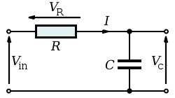Series RC circuit

By viewing the circuit as a voltage divider, the voltage across the capacitor is:

$V_C(s) = \frac{1/Cs}{R + 1/Cs}V_{in}(s) = \frac{1}{1 + RCs}V_{in}(s)$

and the voltage across the resistor is:

$V_R(s) = \frac{R}{R + 1/ Cs}V_{in}(s) = \frac{ RCs}{1 + RCs}V_{in}(s)$.

Transfer functions

The transfer function from the input voltage to the voltage across the capacitor is

$H_C(s) = { V_C(s) \over V_{in}(s) } = { 1 \over 1 + RCs }$.

Similarly, the transfer function from the input to the voltage across the resistor is

$H_R(s) = { V_R(s) \over V_{in}(s) } = { RCs \over 1 + RCs }$.

Poles and zeros

Both transfer functions have a single pole located at

$s = - {1 \over RC }$ .

In addition, the transfer function for the resistor has a zero located at the origin.

Gain and phase angle

The magnitude of the gains across the two components are:

$G_C = | H_C(j \omega) | = \left|\frac{V_C(j \omega)}{V_{in}(j \omega)}\right| = \frac{1}{\sqrt{1 + \left(\omega RC\right)^2}}$

and

$G_R = | H_R(j \omega) | = \left|\frac{V_R(j \omega)}{V_{in}(j \omega)}\right| = \frac{\omega RC}{\sqrt{1 + \left(\omega RC\right)^2}}$,

and the phase angles are:

$\phi_C = \angle H_C(j \omega) = \tan^{-1}\left(-\omega RC\right)$

and

$\phi_R = \angle H_R(j \omega) = \tan^{-1}\left(\frac{1}{\omega RC}\right)$.

These expressions together may be substituted into the usual expression for the phasor representing the output:

$V_C \ = \ G_{C}V_{in} e^{j\phi_C}$

$V_R \ = \ G_{R}V_{in} e^{j\phi_R}$.

Current

The current in the circuit is the same everywhere since the circuit is in series:

$I(s) = \frac{V_{in}(s) }{R + \frac{1}{Cs}} = { Cs \over 1 + RCs } V_{in}(s)$

Impulse response

The impulse response for each voltage is the inverse Laplace transform of the corresponding transfer function. It represents the response of the circuit to an input voltage consisting of an impulse or Dirac delta function.

The impulse response for the capacitor voltage is

$h_C(t) = {1 \over RC} e^{-t / RC} u(t) = { 1 \over \tau} e^{-t / \tau} u(t)$

where u(t) is the Heaviside step function and

$\tau \ = \ RC$

is the time constant.

Similarly, the impulse response for the resistor voltage is

$h_R(t) = \delta (t) - {1 \over RC} e^{-t / RC} u(t) = \delta (t) - { 1 \over \tau} e^{-t / \tau} u(t)$

where δ(t) is the Dirac delta function

Frequency-domain considerations

These are frequency domain expressions. Analysis of them will show which frequencies the circuits (or filters) pass and reject. This analysis rests on a consideration of what happens to these gains as the frequency becomes very large and very small.

As $\omega \to \infty$:

$G_C \to 0$

$G_R \to 1$.

As $\omega \to 0$:

$G_C \to 1$

$G_R \to 0$.

This shows that, if the output is taken across the capacitor, high frequencies are attenuated (rejected) and low frequencies are passed. Thus, the circuit behaves as a low-pass filter. If, though, the output is taken across the resistor, high frequencies are passed and low frequencies are rejected. In this configuration, the circuit behaves as a high-pass filter.

The range of frequencies that the filter passes is called its bandwidth. The point at which the filter attenuates the signal to half its unfiltered power is termed its cutoff frequency. This requires that the gain of the circuit be reduced to

$G_C = G_R = \frac{1}{\sqrt{2}}$.

Solving the above equation yields

$\omega_{c} = \frac{1}{RC} \ \mathrm{rad/s}$

or

$f_c = \frac{1}{2\pi RC} \ \mathrm{Hz}$

which is the frequency that the filter will attenuate to half its original power.

Clearly, the phases also depend on frequency, although this effect is less interesting generally than the gain variations.

As $\omega \to 0$:

$\phi_C \to 0$

$\phi_R \to 90^{\circ} = \pi/2^{c}$.

As $\omega \to \infty$:

$\phi_C \to -90^{\circ} = -\pi/2^{c}$

$\phi_R \to 0$

So at DC (0 Hz), the capacitor voltage is in phase with the signal voltage while the resistor voltage leads it by 90°. As frequency increases, the capacitor voltage comes to have a 90° lag relative to the signal and the resistor voltage comes to be in-phase with the signal.

Time-domain considerations

This section relies on knowledge of e, the natural logarithmic constant.

The most straightforward way to derive the time domain behaviour is to use the Laplace transforms of the expressions for V_C and V_R given above. This effectively transforms $j\omega \to s$. Assuming a step input (i.e. V_in = 0 before t = 0 and then V_in = V afterwards):

$V_{in}(s) = V\frac{1}{s}$

$V_C(s) = V\frac{1}{1 + sRC}\frac{1}{s}$

and

$V_R(s) = V\frac{sRC}{1 + sRC}\frac{1}{s}$.

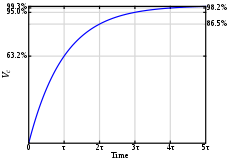Capacitor voltage step-response.

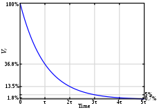Resistor voltage step-response.

Partial fractions expansions and the inverse Laplace transform yield:

$\,\!V_C(t) = V\left(1 - e^{-t/RC}\right)$

$\,\!V_R(t) = Ve^{-t/RC}$.

These equations are for calculating the voltage across the capacitor and resistor respectively while the capacitor is charging; for discharging, the equations are vice-versa. These equations can be rewritten in terms of charge and current using the relationships C=Q/V and V=IR (see Ohm's law).

Thus, the voltage across the capacitor tends towards V as time passes, while the voltage across the resistor tends towards 0, as shown in the figures. This is in keeping with the intuitive point that the capacitor will be charging from the supply voltage as time passes, and will eventually be fully charged.

These equations show that a series RC circuit has a time constant, usually denoted τ = RC being the time it takes the voltage across the component to either rise (across C) or fall (across R) to within 1 / e of its final value. That is, τ is the time it takes V_C to reach V(1 − 1 / e) and V_R to reach V(1 / e).

The rate of change is a fractional $\left(1 - \frac{1}{e}\right)$ per τ. Thus, in going from t = Nτ to t = (N + 1)τ, the voltage will have moved about 63.2 % of the way from its level at t = Nτ toward its final value. So C will be charged to about 63.2 % after τ, and essentially fully charged (99.3 %) after about 5τ. When the voltage source is replaced with a short-circuit, with C fully charged, the voltage across C drops exponentially with t from V towards 0. C will be discharged to about 36.8 % after τ, and essentially fully discharged (0.7 %) after about 5τ. Note that the current, I, in the circuit behaves as the voltage across R does, via Ohm's Law.

These results may also be derived by solving the differential equations describing the circuit:

$\frac{V_{in} - V_C}{R} = C\frac{dV_C}{dt}$

and

$\,\!V_R = V_{in} - V_C$.

The first equation is solved by using an integrating factor and the second follows easily; the solutions are exactly the same as those obtained via Laplace transforms.

Integrator

Consider the output across the capacitor at high frequency i.e.

$\omega \gg \frac{1}{RC}$.

This means that the capacitor has insufficient time to charge up and so its voltage is very small. Thus the input voltage approximately equals the voltage across the resistor. To see this, consider the expression for I given above:

$I = \frac{V_{in}}{R+1/j\omega C}$

but note that the frequency condition described means that

$\omega C \gg \frac{1}{R}$

so

$I \approx \frac{V_{in}}{R}$ which is just Ohm's Law.

Now,

$V_C = \frac{1}{C}\int_{0}^{t}Idt$

so

$V_C \approx \frac{1}{RC}\int_{0}^{t}V_{in}dt$,

which is an integrator across the capacitor.

Differentiator

Consider the output across the resistor at low frequency i.e.,

$\omega \ll \frac{1}{RC}$.

This means that the capacitor has time to charge up until its voltage is almost equal to the source's voltage. Considering the expression for I again, when

$R \ll \frac{1}{\omega C}$,

so

$I \approx \frac{V_{in}}{1/j\omega C}$

$V_{in} \approx \frac{I}{j\omega C} = V_C$

Now,

$V_R = IR = C\frac{dV_C}{dt}R$

$V_R \approx RC\frac{dV_{in}}{dt}$

which is a differentiator across the resistor.

More accurate integration and differentiation can be achieved by placing resistors and capacitors as appropriate on the input and feedback loop of operational amplifiers (see operational amplifier integrator and operational amplifier differentiator).

Parallel circuit

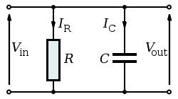Parallel RC circuit

The parallel RC circuit is generally of less interest than the series circuit. This is largely because the output voltage V_out is equal to the input voltage V_in — as a result, this circuit does not act as a filter on the input signal unless fed by a current source.

With complex impedances:

$I_R = \frac{V_{in}}{R}\,$

and

$I_C = j\omega C V_{in}\,$.

This shows that the capacitor current is 90° out of phase with the resistor (and source) current. Alternatively, the governing differential equations may be used:

$I_R = \frac{V_{in}}{R}$

and

$I_C = C\frac{dV_{in}}{dt}$.

When fed by a current source, the transfer function of a parallel RC circuit is

$\frac{V_{out}}{I_{in}} = \frac{R}{1+sRC}$.

See also

• RL circuit
• LC circuit
• RLC circuit
• Electrical network
• List of electronics topics
• Step response
• RC Circuit and continuous-repayment mortgage

External links

• RC Filter Calculator