- Chebyshev filter
-
Linear analog electronic filters - Butterworth filter
- Chebyshev filter
- Elliptic (Cauer) filter
- Bessel filter
- Gaussian filter
- Optimum "L" (Legendre) filter
- Linkwitz-Riley filter
Simple filtersedit Chebyshev filters are analog or digital filters having a steeper roll-off and more passband ripple (type I) or stopband ripple (type II) than Butterworth filters. Chebyshev filters have the property that they minimize the error between the idealized and the actual filter characteristic over the range of the filter, but with ripples in the passband. This type of filter is named in honor of Pafnuty Chebyshev because its mathematical characteristics are derived from Chebyshev polynomials.
Because of the passband ripple inherent in Chebyshev filters, the ones that have a smoother response in the passband but a more irregular response in the stopband are preferred for some applications.
Contents
Type I Chebyshev filters
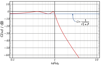 The frequency response of a fourth-order type I Chebyshev low-pass filter with ε = 1
These are the most common Chebyshev filters. The gain (or amplitude) response as a function of angular frequency ω of the nth-order low-pass filter is
where ε is the ripple factor, ω0 is the cutoff frequency and Tn() is a Chebyshev polynomial of the nth order.
The passband exhibits equiripple behavior, with the ripple determined by the ripple factor ε. In the passband, the Chebyshev polynomial alternates between 0 and 1 so the filter gain will alternate between maxima at G = 1 and minima at
 . At the cutoff frequency ω0 the gain again has the value
  but continues to drop into the stop band as the frequency increases. This behavior is shown in the diagram on the right. The common practice of defining the cutoff frequency at −3 dB is usually not applied to Chebyshev filters; instead the cutoff is taken as the point at which the gain falls to the value of the ripple for the final time.
The order of a Chebyshev filter is equal to the number of reactive components (for example, inductors) needed to realize the filter using analog electronics.
The ripple is often given in dB:
- Ripple in dB =

so that a ripple amplitude of 3 dB results from ε = 1.
An even steeper roll-off can be obtained if we allow for ripple in the stop band, by allowing zeroes on the jω-axis in the complex plane. This will however result in less suppression in the stop band. The result is called an elliptic filter, also known as Cauer filter.
Poles and zeroes
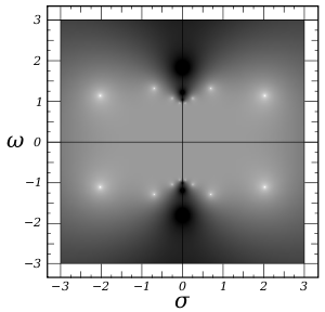
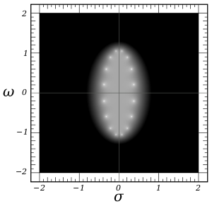 Log of the absolute value of the gain of an 8th order Chebyshev type I filter in complex frequency space (s = σ + jω) with ε = 0.1 and ω0 = 1. The white spots are poles and are arranged on an ellipse with a semi-axis of 0.3836... in σ and 1.071... in ω. The transfer function poles are those poles in the left half plane. Black corresponds to a gain of 0.05 or less, white corresponds to a gain of 20 or more.
For simplicity, assume that the cutoff frequency is equal to unity. The poles (ωpm) of the gain of the Chebyshev filter will be the zeroes of the denominator of the gain. Using the complex frequency s:
Defining − js = cos(θ) and using the trigonometric definition of the Chebyshev polynomials yields:
Solving for θ
where the multiple values of the arc cosine function are made explicit using the integer index m. The poles of the Chebyshev gain function are then:
Using the properties of the trigonometric and hyperbolic functions, this may be written in explicitly complex form:
where m = 1, 2,..., n and
This may be viewed as an equation parametric in θn and it demonstrates that the poles lie on an ellipse in s-space centered at s = 0 with a real semi-axis of length sinh(arsinh(1 / ε) / n) and an imaginary semi-axis of length of cosh(arsinh(1 / ε) / n).
The transfer function
The above expression yields the poles of the gain G. For each complex pole, there is another which is the complex conjugate, and for each conjugate pair there are two more that are the negatives of the pair. The transfer function must be stable, so that its poles will be those of the gain that have negative real parts and therefore lie in the left half plane of complex frequency space. The transfer function is then given by
where
 are only those poles with a negative sign in front of the real term in the above equation for the poles.
The group delay
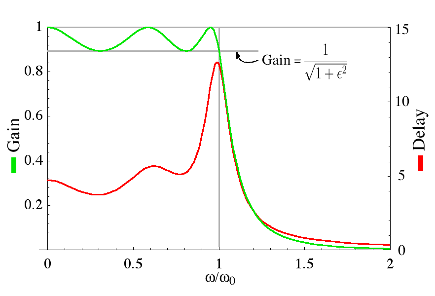
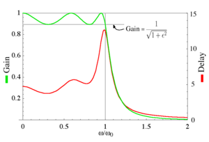 Gain and group delay of a fifth-order type I Chebyshev filter with ε = 0.5.
The group delay is defined as the derivative of the phase with respect to angular frequency and is a measure of the distortion in the signal introduced by phase differences for different frequencies.
The gain and the group delay for a fifth-order type I Chebyshev filter with ε=0.5 are plotted in the graph on the left. It can be seen that there are ripples in the gain and the group delay in the passband but not in the stopband.
Type II Chebyshev filters
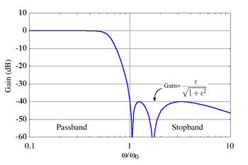 The frequency response of a fifth-order type II Chebyshev low-pass filter with
Also known as inverse Chebyshev, this type is less common because it does not roll off as fast as type I, and requires more components. It has no ripple in the passband, but does have equiripple in the stopband. The gain is:
In the stopband, the Chebyshev polynomial will oscillate between 0 and 1 so that the gain will oscillate between zero and
and the smallest frequency at which this maximum is attained will be the cutoff frequency ωo. The parameter ε is thus related to the stopband attenuation γ in decibels by:
For a stopband attenuation of 5dB, ε = 0.6801; for an attenuation of 10dB, ε = 0.3333. The frequency fC = ωC/2π is the cutoff frequency. The 3dB frequency fH is related to fC by:
Poles and zeroes
 Log of the absolute value of the gain of an 8th order Chebyshev type II filter in complex frequency space (s=σ+jω) with ε = 0.1 and ω0 = 1. The white spots are poles and the black spots are zeroes. All 16 poles are shown. Each zero has multiplicity of two, and 12 zeroes are shown and four are located outside the picture, two on the positive ω axis, and two on the negative. The poles of the transfer function will be poles on the left half plane and the zeroes of the transfer function will be the zeroes, but with multiplicity 1. Black corresponds to a gain of 0.05 or less, white corresponds to a gain of 20 or more.
Again, assuming that the cutoff frequency is equal to unity, the poles (ωpm) of the gain of the Chebyshev filter will be the zeroes of the denominator of the gain:
The poles of gain of the type II Chebyshev filter will be the inverse of the poles of the type I filter:
where m = 1, 2, ..., n . The zeroes (ωzm) of the type II Chebyshev filter will be the zeroes of the numerator of the gain:
The zeroes of the type II Chebyshev filter will thus be the inverse of the zeroes of the Chebyshev polynomial.
for m = 1, 2, ..., n.
The transfer function
The transfer function will be given by the poles in the left half plane of the gain function, and will have the same zeroes but these zeroes will be single rather than double zeroes.
The group delay
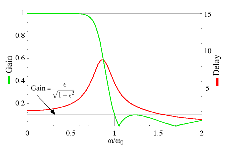
 Gain and group delay of a fifth-order type II Chebyshev filter with ε = 0.1.
The gain and the group delay for a fifth-order type II Chebyshev filter with ε=0.1 are plotted in the graph on the left. It can be seen that there are ripples in the gain in the stop band but not in the pass band.
Implementation
Cauer topology
A passive LC Chebyshev low-pass filter may be realized using a Cauer topology. Inductor or capacitor values of a nth-order Chebyshev filter may be calculated from the following equations:
- G1, Gk are the capacitor or inductor element values.
- fH, the 3 dB frequency is calculated with:

- The coefficients A, Y, β, Ak, and Bk may be calculated from the following equations:
-

- where RdB is the passband ripple in decibels.
 Low-pass filter using Cauer topology
The calculated Gk values may then be converted into shunt capacitors and top inductors as shown on the right, or they may be converted into top capacitors and shunt inductors.
- For example, C1 shunt = G1, L2 top = G2, ...
- or L1 shunt = G1, C1 top = G2, ...
The resulting circuit is a normalized low-pass filter. Using frequency transformations and impedance scaling, the normalized low-pass filter may be transformed into high-pass, band-pass, and band-stop filters of any desired cutoff frequency or bandwidth.
Digital
As with most analog filters, the Chebyshev may be converted to a digital (discrete-time) recursive form via the bilinear transform. However, as digital filters have a finite bandwidth, the response shape of the transformed Chebyshev will be warped. Alternatively, the Matched Z-transform method may be used, which does not warp the response.
Comparison with other linear filters
Here is an image showing the Chebyshev filters next to other common kind of filters obtained with the same number of coefficients (all filters are fifth order):
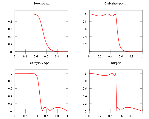
As is clear from the image, Chebyshev filters are sharper than the Butterworth filter; they are not as sharp as the elliptic one, but they show fewer ripples over the bandwidth.
See also
- Chebyshev nodes
- Chebyshev polynomial
References
- Daniels, Richard W. (1974). Approximation Methods for Electronic Filter Design. New York: McGraw-Hill. ISBN 0-07-015308-6.
- Williams, Arthur B.; Taylors, Fred J. (1988). Electronic Filter Design Handbook. New York: McGraw-Hill. ISBN 0-07-070434-1
Categories:- Linear filters
- Network synthesis filters
- Electronic design


Wikimedia Foundation. 2010.