Digital filter

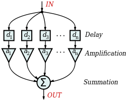A general finite impulse response filter with n stages, each with an independent delay, d_i, and amplification gain, a_i.

In electronics, computer science and mathematics, a digital filter is a system that performs mathematical operations on a sampled, discrete-time signal to reduce or enhance certain aspects of that signal. This is in contrast to the other major type of electronic filter, the analog filter, which is an electronic circuit operating on continuous-time analog signals. An analog signal may be processed by a digital filter by first being digitized and represented as a sequence of numbers, then manipulated mathematically, and then reconstructed as a new analog signal (see digital signal processing). In an analog filter, the input signal is "directly" manipulated by the circuit.

A digital filter system usually consists of an analog-to-digital converter to sample the input signal, followed by a microprocessor and some peripheral components such as memory to store data and filter coefficients etc. Finally a digital-to-analog converter to complete the output stage. Program Instructions (software) running on the microprocessor implement the digital filter by performing the necessary mathematical operations on the numbers received from the ADC. In some high performance applications, an FPGA or ASIC is used instead of a general purpose microprocessor, or a specialized DSP with specific paralleled architecture for expediting operations such as filtering.

Digital filters may be more expensive than an equivalent analog filter due to their increased complexity, but they make practical many designs that are impractical or impossible as analog filters. Since digital filters use a sampling process and discrete-time processing, they experience latency (the difference in time between the input and the response), which is almost irrelevant in analog filters.

Digital filters are commonplace and an essential element of everyday electronics such as radios, cellphones, and stereo receivers.

Characterization of digital filters

A digital filter is characterized by its transfer function, or equivalently, its difference equation. Mathematical analysis of the transfer function can describe how it will respond to any input. As such, designing a filter consists of developing specifications appropriate to the problem (for example, a second-order low pass filter with a specific cut-off frequency), and then producing a transfer function which meets the specifications.

The transfer function for a linear, time-invariant, digital filter can be expressed as a transfer function in the Z-domain; if it is causal, then it has the form:

$H(z) = \frac{B(z)}{A(z)} = \frac{{b_{0}+b_{1}z^{-1}+b_{2}z^{-2} + \cdots + b_{N}z^{-N}}}{{1+a_{1}z^{-1}+a_{2}z^{-2} + \cdots +a_{M}z^{-M}}}$

where the order of the filter is the greater of N or M. See Z-transform's LCCD equation for further discussion of this transfer function.

This is the form for a recursive filter with both the inputs (Numerator) and outputs (Denominator), which typically leads to an IIR infinite impulse response behaviour, but if the denominator is made equal to unity i.e. no feedback, then this becomes an FIR or finite impulse response filter.

Analysis techniques

A variety of mathematical techniques may be employed to analyze the behaviour of a given digital filter. Many of these analysis techniques may also be employed in designs, and often form the basis of a filter specification.

Typically, one analyzes filters by calculating how the filter will respond to a simple input such as an impulse response. One can then extend this information to visualize the filter's response to more complex signals. Riemann spheres have been used, together with digital video, for this purpose.

Impulse response

The impulse response, often denoted h[k] or h_k, is a measurement of how a filter will respond to the Kronecker delta function. For example, given a difference equation, one would set x₀ = 1 and x_k = 0 for $k \ne 0$ and evaluate. The impulse response is a characterization of the filter's behaviour. Digital filters are typically considered in two categories: infinite impulse response (IIR) and finite impulse response (FIR). In the case of linear time-invariant FIR filters, the impulse response is exactly equal to the sequence of filter coefficients:

$\ y_n= \sum_{k=0}^{n-1} h_{k} x_{n-k}$

IIR filters on the other hand are recursive, with the output depending on both current and previous inputs as well as previous outputs. The general form of the an IIR filter is thus:

$\ \sum_{m=0}^{M-1} a_{m}y_{n-m} = \sum_{k=0}^{n-1} b_{k} x_{n-k}$

Plotting the impulse response will reveal how a filter will respond to a sudden, momentary disturbance.

Difference equation

In discrete-time systems, the digital filter is often implemented by converting the transfer function to a linear constant-coefficient difference equation (LCCD) via the Z-transform. The discrete frequency-domain transfer function is written as the ratio of two polynomials. For example:

$H(z) = \frac{(z+1)^2} {(z-\frac{1}{2}) (z+\frac{3}{4})}$

This is expanded:

$H(z) = \frac{z^2+ 2z +1} {z^2 +\frac{1}{4} z - \frac{3}{8}}$

and divided by the highest order of z:

$H(z) = \frac{1 + 2z^{-1} +z^{-2}} {1 +\frac{1}{4} z^{-1} - \frac{3}{8} z^{-2}} = \frac{Y(z)}{X(z)}$

The coefficients of the denominator, a_k, are the 'feed-backward' coefficients and the coefficients of the numerator are the 'feed-forward' coefficients, b_k. The resultant linear difference equation is:

$y[n] = -\sum_{k=1}^{N} a_{k} y[n-k] + \sum_{k=0}^{M} b_{k} x[n-k]$

or, for the example above:

$\frac{Y(z)}{X(z)} = \frac{1 + 2z^{-1} +z^{-2}} {1 +\frac{1}{4} z^{-1} - \frac{3}{8} z^{-2}}$

rearranging terms:

$\Rightarrow (1 +\frac{1}{4} z^{-1} - \frac{3}{8} z^{-2}) Y(z) = (1 + 2z^{-1} +z^{-2}) X(z)$

then by taking the inverse z-transform:

$\Rightarrow y[n] + \frac{1}{4} y[n-1] - \frac{3}{8} y[n-2] = x[n] + 2x[n-1] + x[n-2]$

and finally, by solving for y[n]:

$y[n] = - \frac{1}{4} y[n-1] + \frac{3}{8} y[n-2] + x[n] + 2x[n-1] + x[n-2]$

This equation shows how to compute the next output sample, y[n], in terms of the past outputs, y[n − p], the present input, x[n], and the past inputs, x[n − p]. Applying the filter to an input in this form is equivalent to a Direct Form I or II realization, depending on the exact order of evaluation.

Filter design

Main article: Filter design

The design of digital filters is a deceptively complex topic.^[1] Although filters are easily understood and calculated, the practical challenges of their design and implementation are significant and are the subject of much advanced research.

There are two categories of digital filter: the recursive filter and the nonrecursive filter. These are often referred to as infinite impulse response (IIR) filters and finite impulse response (FIR) filters, respectively.^[2]

Filter realization

After a filter is designed, it must be realized by developing a signal flow diagram that describes the filter in terms of operations on sample sequences.

A given transfer function may be realized in many ways. Consider how a simple expression such as ax + bx + c could be evaluated – one could also compute the equivalent x(a + b) + c. In the same way, all realizations may be seen as "factorizations" of the same transfer function, but different realizations will have different numerical properties. Specifically, some realizations are more efficient in terms of the number of operations or storage elements required for their implementation, and others provide advantages such as improved numerical stability and reduced round-off error. Some structures are better for fixed-point arithmetic and others may be better for floating-point arithmetic.

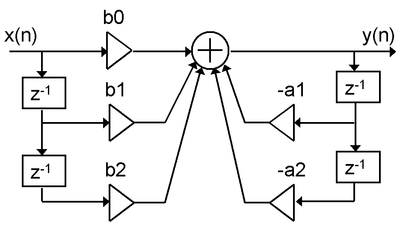
Direct Form I

A straightforward approach for IIR filter realization is Direct Form I, where the difference equation is evaluated directly. This form is practical for small filters, but may be inefficient and impractical (numerically unstable) for complex designs.^[3] In general, this form requires 2N delay elements (for both input and output signals) for a filter of order N.

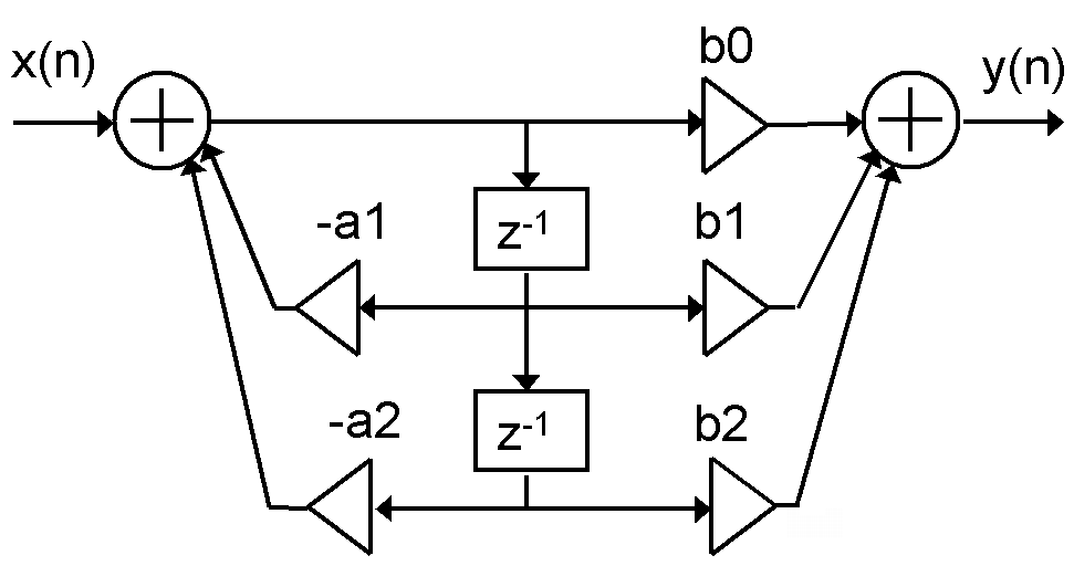
Direct Form II

The alternate Direct Form II only needs N delay units, where N is the order of the filter – potentially half as much as Direct Form I. This structure is obtained by reversing the order of the numerator and denominator sections of Direct Form I, since they are in fact two linear systems, and the commutativity property applies. Then, one will notice that there are two columns of delays (z ^{− 1}) that tap off the center net, and these can be combined since they are redundant, yielding the implementation as shown below.

The disadvantage is that Direct Form II increases the possibility of arithmetic overflow for filters of high Q or resonance.^[4] It has been shown that as Q increases, the round-off noise of both direct form topologies increases without bounds.^[5] This is because, conceptually, the signal is first passed through an all-pole filter (which normally boosts gain at the resonant frequencies) before the result of that is saturated, then passed through an all-zero filter (which often attenuates much of what the all-pole half amplifies).

Cascaded second-order sections

A common strategy is to realize a higher-order (greater than 2) digital filter as a cascaded series of second-order "biquadratric" (or "biquad") sections^[6] (see digital biquad filter). Advantages of this strategy is that the coefficient range is limited. Cascading direct form II sections result in N delay elements for filter order of N. Cascading direct form I sections result in N+2 delay elements since the delay elements of the input of any section (except the first section) are a redundant with the delay elements of the output of the preceding section.

Other Forms

Other forms include:

• Direct Form I and II transpose
• Series/cascade^[7]
• Parallel^[7]
• Ladder form^[7]
• Lattice form^[7]
• Coupled normal form
• Multifeedback
• Analog-inspired forms such as Sallen-key and state variable filters
• Systolic arrays

Comparison of analog and digital filters

Digital filters are not subject to the component non-linearities that greatly complicate the design of analog filters. Analog filters consist of imperfect electronic components, whose values are specified to a limit tolerance (e.g. resistor values often have a tolerance of +/- 5%) and which may also change with temperature and drift with time. As the order of an analog filter increases, and thus its component count, the effect of variable component errors is greatly magnified. In digital filters, the coefficient values are stored in computer memory, making them far more stable and predictable.^[8]

Because the coefficients of digital filters are definite, they can be used to achieve much more complex and selective designs – specifically with digital filters, one can achieve a lower passband ripple, faster transition, and higher stopband attenuation than is practical with analog filters. Even if the design could be achieved using analog filters, the engineering cost of designing an equivalent digital filter would likely be much lower. Furthermore, one can readily modify the coefficients of a digital filter to make an adaptive filter or a user-controllable parametric filter. While these techniques are possible in an analog filter, they are again considerably more difficult.

Digital filters can be used in the design of finite impulse response filters. Analog filters do not have the same capability, because finite impulse response filters require delay elements.

Digital filters rely less on analog circuitry, potentially allowing for a better signal-to-noise ratio. A digital filter will introduce noise to a signal during analog low pass filtering, analog to digital conversion, digital to analog conversion and may introduce digital noise due to quantization. With analog filters, every component is a source of thermal noise (such as Johnson noise), so as the filter complexity grows, so does the noise.

However, digital filters do introduce a higher fundamental latency to the system. In an analog filter, latency is often negligible; strictly speaking it is the time for an electrical signal to propagate through the filter circuit. In digital filters, latency is a function of the number of delay elements in the system.

Digital filters also tend to be more limited in bandwidth than analog filters. High bandwidth digital filters require expensive ADC/DACs and fast computer hardware for processing.

In very simple cases, it is more cost effective to use an analog filter. Introducing a digital filter requires considerable overhead circuitry, as previously discussed, including two low pass analog filters.

Types of digital filters

Many digital filters are based on the Fast Fourier transform, a mathematical algorithm that quickly extracts the frequency spectrum of a signal, allowing the spectrum to be manipulated (such as to create band-pass filters) before converting the modified spectrum back into a time-series signal.

Another form of a digital filter is that of a state-space model. A well used state-space filter is the Kalman filter published by Rudolf Kalman in 1960.

See also

• Bessel filter
• Butterworth filter
• Elliptical filter (Cauer filter)
• Linkwitz-Riley filter
• Chebyshev filter
• Ladder filter
• Sample (signal)
• Electronic filter
• Filter design
• Biquad filter
• High-pass filter, Low-pass filter
• Infinite impulse response, Finite impulse response
• Bilinear transform

References

General

• A. Antoniou, Digital Filters: Analysis, Design, and Applications, New York, NY: McGraw-Hill, 1993.
• J. O. Smith III, Introduction to Digital Filters with Audio Applications, Center for Computer Research in Music and Acoustics (CCRMA), Stanford University, September 2007 Edition.
• S.K. Mitra, Digital Signal Processing: A Computer-Based Approach, New York, NY: McGraw-Hill, 1998.
• A.V. Oppenheim and R.W. Schafer, Discrete-Time Signal Processing, Upper Saddle River, NJ: Prentice-Hall, 1999.
• J.F. Kaiser, Nonrecursive Digital Filter Design Using the Io-sinh Window Function, Proc. 1974 IEEE Int. Symp. Circuit Theory, pp. 20–23, 1974.
• S.W.A. Bergen and A. Antoniou, Design of Nonrecursive Digital Filters Using the Ultraspherical Window Function, EURASIP Journal on Applied Signal Processing, vol. 2005, no. 12, pp. 1910–1922, 2005.
• T.W. Parks and J.H. McClellan, Chebyshev Approximation for Nonrecursive Digital Filters with Linear Phase, IEEE Trans. Circuit Theory, vol. CT-19, pp. 189–194, Mar. 1972.
• L. R. Rabiner, J.H. McClellan, and T.W. Parks, FIR Digital Filter Design Techniques Using Weighted Chebyshev Approximation, Proc. IEEE, vol. 63, pp. 595–610, Apr. 1975.
• A.G. Deczky, Synthesis of Recursive Digital Filters Using the Minimum p-Error Criterion, IEEE Trans. Audio Electroacoust., vol. AU-20, pp. 257–263, Oct. 1972.

Cited

1. ^ M. E. Valdez, Digital Filters, 2001.
2. ^ A. Antoniou, chapter 1
3. ^ J. O. Smith III, Direct Form I
4. ^ J. O. Smith III, Direct Form II
5. ^ L. B. Jackson, "On the Interaction of Roundoff Noise and Dynamic Range in Digital Filters," Bell Sys. Tech. J., vol. 49 (1970 Feb.), reprinted in Digital Signal Process, L. R. Rabiner and C. M. Rader, Eds. (IEEE Press, New York, 1972).
6. ^ J. O. Smith III, Series Second Order Sections
7. ^ ^{a b c d} A. Antoniou
8. ^ http://www.dspguide.com/ch21/1.htm

External links

• WinFilter – Free filter design software
• Filtplot – Free customizable digital filter design software built with python and boost (WinXP/Ubuntu 6.10/RHEL-4). Also with interactive web interface.
• DISPRO – Free filter design software
• Java demonstration of digital filters
• IIR Explorer educational software
• Introduction to Filtering
• Introduction to Digital Filters
• Publicly available, very comprehensive lecture notes on Digital Linear Filtering (see bottom of the page)