Graph coloring

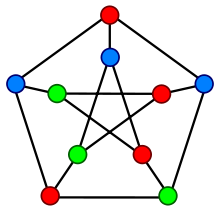A proper vertex coloring of the Petersen graph with 3 colors, the minimum number possible.

In graph theory, graph coloring is a special case of graph labeling; it is an assignment of labels traditionally called "colors" to elements of a graph subject to certain constraints. In its simplest form, it is a way of coloring the vertices of a graph such that no two adjacent vertices share the same color; this is called a vertex coloring. Similarly, an edge coloring assigns a color to each edge so that no two adjacent edges share the same color, and a face coloring of a planar graph assigns a color to each face or region so that no two faces that share a boundary have the same color.

Vertex coloring is the starting point of the subject, and other coloring problems can be transformed into a vertex version. For example, an edge coloring of a graph is just a vertex coloring of its line graph, and a face coloring of a planar graph is just a vertex coloring of its planar dual. However, non-vertex coloring problems are often stated and studied as is. That is partly for perspective, and partly because some problems are best studied in non-vertex form, as for instance is edge coloring.

The convention of using colors originates from coloring the countries of a map, where each face is literally colored. This was generalized to coloring the faces of a graph embedded in the plane. By planar duality it became coloring the vertices, and in this form it generalizes to all graphs. In mathematical and computer representations it is typical to use the first few positive or nonnegative integers as the "colors". In general one can use any finite set as the "color set". The nature of the coloring problem depends on the number of colors but not on what they are.

Graph coloring enjoys many practical applications as well as theoretical challenges. Beside the classical types of problems, different limitations can also be set on the graph, or on the way a color is assigned, or even on the color itself. It has even reached popularity with the general public in the form of the popular number puzzle Sudoku. Graph coloring is still a very active field of research.

Note: Many terms used in this article are defined in Glossary of graph theory.

History

See also: History of the four color theorem  and History of graph theory

The first results about graph coloring deal almost exclusively with planar graphs in the form of the coloring of maps. While trying to color a map of the counties of England, Francis Guthrie postulated the four color conjecture, noting that four colors were sufficient to color the map so that no regions sharing a common border received the same color. Guthrie’s brother passed on the question to his mathematics teacher Augustus de Morgan at University College, who mentioned it in a letter to William Hamilton in 1852. Arthur Cayley raised the problem at a meeting of the London Mathematical Society in 1879. The same year, Alfred Kempe published a paper that claimed to establish the result, and for a decade the four color problem was considered solved. For his accomplishment Kempe was elected a Fellow of the Royal Society and later President of the London Mathematical Society.^[1]

In 1890, Heawood pointed out that Kempe’s argument was wrong. However, in that paper he proved the five color theorem, saying that every planar map can be colored with no more than five colors, using ideas of Kempe. In the following century, a vast amount of work and theories were developed to reduce the number of colors to four, until the four color theorem was finally proved in 1976 by Kenneth Appel and Wolfgang Haken. Perhaps surprisingly, the proof went back to the ideas of Heawood and Kempe and largely disregarded the intervening developments.^[2] The proof of the four color theorem is also noteworthy for being the first major computer-aided proof.

In 1912, George David Birkhoff introduced the chromatic polynomial to study the coloring problems, which was generalised to the Tutte polynomial by Tutte, important structures in algebraic graph theory. Kempe had already drawn attention to the general, non-planar case in 1879,^[3] and many results on generalisations of planar graph coloring to surfaces of higher order followed in the early 20th century.

In 1960, Claude Berge formulated another conjecture about graph coloring, the strong perfect graph conjecture, originally motivated by an information-theoretic concept called the zero-error capacity of a graph introduced by Shannon. The conjecture remained unresolved for 40 years, until it was established as the celebrated strong perfect graph theorem in 2002 by Chudnovsky, Robertson, Seymour, Thomas 2002.

Graph coloring has been studied as an algorithmic problem since the early 1970s: the chromatic number problem is one of Karp’s 21 NP-complete problems from 1972, and at approximately the same time various exponential-time algorithms were developed based on backtracking and on the deletion-contraction recurrence of Zykov (1949). One of the major applications of graph coloring, register allocation in compilers, was introduced in 1981.

Definition and terminology

This graph can be 3-colored in 12 different ways.

Vertex coloring

When used without any qualification, a coloring of a graph is almost always a proper vertex coloring, namely a labelling of the graph’s vertices with colors such that no two vertices sharing the same edge have the same color. Since a vertex with a loop could never be properly colored, it is understood that graphs in this context are loopless.

The terminology of using colors for vertex labels goes back to map coloring. Labels like red and blue are only used when the number of colors is small, and normally it is understood that the labels are drawn from the integers {1,2,3,...}.

A coloring using at most k colors is called a (proper) k-coloring. The smallest number of colors needed to color a graph G is called its chromatic number, χ(G). A graph that can be assigned a (proper) k-coloring is k-colorable, and it is k-chromatic if its chromatic number is exactly k. A subset of vertices assigned to the same color is called a color class, every such class forms an independent set. Thus, a k-coloring is the same as a partition of the vertex set into k independent sets, and the terms k-partite and k-colorable have the same meaning.

Chromatic polynomial

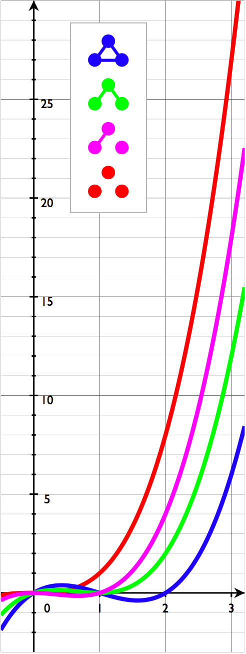
All nonisomorphic graphs on 3 vertices and their chromatic polynomials. The empty graph E₃ (red) admits a 1-coloring, the others admit no such colorings. The green graph admits 12 colorings with 3 colors.

Main article: Chromatic polynomial

The chromatic polynomial counts the number of ways a graph can be colored using no more than a given number of colors. For example, using three colors, the graph in the image to the right can be colored in 12 ways. With only two colors, it cannot be colored at all. With four colors, it can be colored in 24 + 4⋅12 = 72 ways: using all four colors, there are 4! = 24 valid colorings (every assignment of four colors to any 4-vertex graph is a proper coloring); and for every choice of three of the four colors, there are 12 valid 3-colorings. So, for the graph in the example, a table of the number of valid colorings would start like this:

Available colors	1	2	3	4	…
Number of colorings	0	0	12	72	…

The chromatic polynomial is a function P(G, t) that counts the number of t-colorings of G. As the name indicates, for a given G the function is indeed a polynomial in t. For the example graph, P(G, t) = t(t − 1)²(t − 2), and indeed P(G, 4) = 72.

The chromatic polynomial includes at least as much information about the colorability of G as does the chromatic number. Indeed, χ is the smallest positive integer that is not a root of the chromatic polynomial

$\chi (G)=\min\{ k\,\colon\,P(G,k) > 0 \}.$

Chromatic polynomials for certain graphs

Triangle K3	t(t − 1)(t − 2)
Complete graph Kn	$t(t-1)(t-2) \cdots (t-(n-1))$
Tree with n vertices	t(t − 1)n − 1
Cycle Cn	(t − 1)n + ( − 1)n(t − 1)
Petersen graph	t(t − 1)(t − 2)(t7 − 12t6 + 67t5 − 230t4 + 529t3 − 814t2 + 775t − 352)

Edge coloring

Main article: Edge coloring

An edge coloring of a graph is a proper coloring of the edges, meaning an assignment of colors to edges so that no vertex is incident to two edges of the same color. An edge coloring with k colors is called a k-edge-coloring and is equivalent to the problem of partitioning the edge set into k matchings. The smallest number of colors needed for an edge coloring of a graph G is the chromatic index, or edge chromatic number, χ′(G). A Tait coloring is a 3-edge coloring of a cubic graph. The four color theorem is equivalent to the assertion that every planar cubic bridgeless graph admits a Tait coloring.

Properties

Bounds on the chromatic number

Assigning distinct colors to distinct vertices always yields a proper coloring, so

$1 \le \chi(G) \le n.\,$

The only graphs that can be 1-colored are edgeless graphs, and the complete graph K_n of n vertices requires χ(K_n) = n colors. In an optimal coloring there must be at least one of the graph‘s m edges between every pair of color classes, so

$\chi(G)(\chi(G)-1) \le 2m.\,$

If G contains a clique of size k, then at least k colors are needed to color that clique; in other words, the chromatic number is at least the clique number:

$\chi(G) \ge \omega(G).\,$

For interval graphs this bound is tight.

The 2-colorable graphs are exactly the bipartite graphs, including trees and forests. By the four color theorem, every planar graph can be 4-colored.

A greedy coloring shows that every graph can be colored with one more color than the maximum vertex degree,

$\chi(G) \le \Delta(G) + 1. \,$

Complete graphs have χ(G) = n and Δ(G) = n − 1, and odd cycles have χ(G) = 3 and Δ(G) = 2, so for these graphs this bound is best possible. In all other cases, the bound can be slightly improved; Brooks’ theorem^[4] states that

Brooks’ theorem: $\chi (G) \le \Delta (G)$ for a connected, simple graph G, unless G is a complete graph or an odd cycle.

Graphs with high chromatic number

Graphs with large cliques have high chromatic number, but the opposite is not true. The Grötzsch graph is an example of a 4-chromatic graph without a triangle, and the example can be generalised to the Mycielskians.

Mycielski’s Theorem (Jan Mycielski 1955): There exist triangle-free graphs with arbitrarily high chromatic number.

From Brooks’s theorem, graphs with high chromatic number must have high maximum degree. Another local property that leads to high chromatic number is the presence of a large clique. But colorability is not an entirely local phenomenon: A graph with high girth looks locally like a tree, because all cycles are long, but its chromatic number need not be 2:

Theorem (Erdős): There exist graphs of arbitrarily high girth and chromatic number.

Bounds on the chromatic index

An edge coloring of G is a vertex coloring of its line graph L(G), and vice versa. Thus,

$\chi'(G)=\chi(L(G)). \,$

There is a strong relationship between edge colorability and the graph’s maximum degree Δ(G). Since all edges incident to the same vertex need their own color, we have

$\chi'(G) \ge \Delta(G).\,$

Moreover,

König’s theorem: χ'(G) = Δ(G) if G is bipartite.

In general, the relationship is even stronger than what Brooks’s theorem gives for vertex coloring:

Vizing’s Theorem: A graph of maximal degree Δ has edge-chromatic number Δ or Δ + 1.

Other properties

For planar graphs, vertex colorings are essentially dual to nowhere-zero flows.

About infinite graphs, much less is known. The following is one of the few results about infinite graph coloring:

If all finite subgraphs of an infinite graph G are k-colorable, then so is G, under the assumption of the axiom of choice (de Bruijn & Erdős 1951).

Also, if a graph admits a full n-coloring for every n ≥ n₀, it admits an infinite full coloring (Fawcett 1978).

Open problems

The chromatic number of the plane, where two points are adjacent if they have unit distance, is unknown, although it is one of 4, 5, 6, or 7. Other open problems concerning the chromatic number of graphs include the Hadwiger conjecture stating that every graph with chromatic number k has a complete graph on k vertices as a minor, the Erdős–Faber–Lovász conjecture bounding the chromatic number of unions of complete graphs that have at exactly one vertex in common to each pair, and the Albertson conjecture that among k-chromatic graphs the complete graphs are the ones with smallest crossing number.

When Birkhoff and Lewis introduced the chromatic polynomial in their attack on the four-color theorem, they conjectured that for planar graphs G, the polymomial P(G,t) has no zeros in the region $[4,\infty)$. Although it is known that such a chromatic polynomial has no zeros in the region $[5,\infty)$ and that $P(G,4) \neq 0$, their conjecture is still unresolved. It also remains an unsolved problem to characterize graphs which have the same chromatic polynomial and to determine which polynomials are chromatic.

Algorithms

Graph coloring
Decision
Name	Graph coloring, vertex coloring, k-coloring
Input	Graph G with n vertices. Integer k
Output	Does G admit a proper vertex coloring with k colors?
Running time	O(2 nn)[5]
Complexity	NP-complete
Reduction from	3-Satisfiability
Garey–Johnson	GT4
Optimisation
Name	Chromatic number
Input	Graph G with n vertices.
Output	χ(G)
Complexity	NP-hard
Approximability	O(n (log n)−3(log log n)2)
Inapproximability	O(n1−ε) unless P = NP
Counting problem
Name	Chromatic polymomial
Input	Graph G with n vertices. Integer k
Output	The number P (G,k) of proper k-colorings of G
Running time	O(2 nn)
Complexity	#P-complete
Approximability	FPRAS for restricted cases
Inapproximability	No PTAS unless P = NP

Polynomial time

Determining if a graph can be colored with 2 colors is equivalent to determining whether or not the graph is bipartite, and thus computable in linear time using breadth-first search. More generally, the chromatic number and a corresponding coloring of perfect graphs can be computed in polynomial time using semidefinite programming. Closed formulas for chromatic polynomial are known for many classes of graphs, such as forest, chordal graphs, cycles, wheels, and ladders, so these can be evaluated in polynomial time.

Exact algorithms

Brute-force search for a k-coloring considers every of the kⁿ assignments of k colors to n vertices and checks for each if it is legal. To compute the chromatic number and the chromatic polynomial, this procedure is used for every $k=1,\ldots,n-1$, impractical for all but the smallest input graphs.

Using dynamic programming and a bound on the number of maximal independent sets, k-colorability can be decided in time and space O(2.445ⁿ).^[6] Using the principle of inclusion–exclusion and Yates’s algorithm for the fast zeta transform, k-colorability can be decided in time O(2ⁿn)^[5] for any k. Faster algorithms are known for 3- and 4-colorability, which can be decided in time O(1.3289ⁿ) ^[7] and O(1.7504ⁿ),^[8] respectively.

Contraction

The contraction G / uv of graph G is the graph obtained by identifying the vertices u and v, removing any edges between them, and replacing them with a single vertex w where any edges that were incident on u or v are redirected to w. This operation plays a major role in the analysis of graph coloring.

The chromatic number satisfies the recurrence relation:

χ(G) = min{χ(G + uv),χ(G / uv)}

due to Zykov (1949), where u and v are nonadjacent vertices, G + uv is the graph with the edge uv added. Several algorithms are based on evaluating this recurrence, the resulting computation tree is sometimes called a Zykov tree. The running time is based on the heuristic for choosing the vertices u and v.

The chromatic polynomial satisfies following recurrence relation

P(G − uv,k) = P(G / uv,k) + P(G,k)

where u and v are adjacent vertices and G − uv is the graph with the edge uv removed. P(G − uv,k) represents the number of possible proper colorings of the graph, when the vertices may have same or different colors. The number of proper colorings therefore come from the sum of two graphs. If the vertices u and v have different colors, then we can as well consider a graph, where u and v are adjacent. If u and v have the same colors, we may as well consider a graph, where u and v are contracted. Tutte’s curiosity about which other graph properties satisfied this recurrence led him to discover a bivariate generalization of the chromatic polynomial, the Tutte polynomial.

The expressions give rise to a recursive procedure, called the deletion–contraction algorithm, which forms the basis of many algorithms for graph coloring. The running time satisfies the same recurrence relation as the Fibonacci numbers, so in the worst case, the algorithm runs in time within a polynomial factor of $((1+\sqrt{5})/2)^{n+m}=O(1.6180^{n+m})$.^[9] The analysis can be improved to within a polynomial factor of the number t(G) of spanning trees of the input graph.^[10] In practice, branch and bound strategies and graph isomorphism rejection are employed to avoid some recursive calls, the running time depends on the heuristic used to pick the vertex pair.

Greedy coloring

Main article: Greedy coloring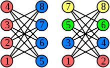

Two greedy colorings of the same graph using different vertex orders. The right example generalises to 2-colorable graphs with n vertices, where the greedy algorithm expends n / 2 colors.

The greedy algorithm considers the vertices in a specific order v₁,…,v_n and assigns to v_i the smallest available color not used by v_i’s neighbours among v₁,…,v_{i − 1}, adding a fresh color if needed. The quality of the resulting coloring depends on the chosen ordering. There exists an ordering that leads to a greedy coloring with the optimal number of χ(G) colors. On the other hand, greedy colorings can be arbitrarily bad; for example, the crown graph on n vertices can be 2-colored, but has an ordering that leads to a greedy coloring with n / 2 colors.

If the vertices are ordered according to their degrees, the resulting greedy coloring uses at most max_i min{d(x_i) + 1,i} colors, at most one more than the graph’s maximum degree. This heuristic is sometimes called the Welsh–Powell algorithm.^[11] Another heuristic due to Brélaz establishes the ordering dynamically while the algorithm proceeds, choosing next the vertex adjacent to the largest number of different colors.^[12] Many other graph coloring heuristics are similarly based on greedy coloring for a specific static or dynamic strategy of ordering the vertices, these algorithms are sometimes called sequential coloring algorithms.

Parallel and distributed algorithms

In the field of distributed algorithms, graph coloring is closely related to the problem of symmetry breaking. The current state-of-the-art randomized algorithms are faster for sufficiently large maximum degree Δ than deterministic algorithms. The fastest randomized algorithms employ the multi-trials technique by Schneider et al.^[13]

In a symmetric graph, a deterministic distributed algorithm cannot find a proper vertex coloring. Some auxiliary information is needed in order to break symmetry. A standard assumption is that initially each node has a unique identifier, for example, from the set {1, 2, ..., n}. Put otherwise, we assume that we are given an n-coloring. The challenge is to reduce the number of colors from n to, e.g., Δ + 1. The more colors are employed, e.g. O(Δ) instead of Δ + 1, the fewer communication rounds are required.^[13]

A straightforward distributed version of the greedy algorithm for (Δ + 1)-coloring requires Θ(n) communication rounds in the worst case − information may need to be propagated from one side of the network to another side.

The simplest interesting case is an n-cycle. Richard Cole and Uzi Vishkin^[14] show that there is a distributed algorithm that reduces the number of colors from n to O(log n) in one synchronous communication step. By iterating the same procedure, it is possible to obtain a 3-coloring of an n-cycle in O(log* n) communication steps (assuming that we have unique node identifiers).

The function log*, iterated logarithm, is an extremely slowly growing function, "almost constant". Hence the result by Cole and Vishkin raised the question of whether there is a constant-time distribute algorithm for 3-coloring an n-cycle. Linial (1992) showed that this is not possible: any deterministic distributed algorithm requires Ω(log* n) communication steps to reduce an n-coloring to a 3-coloring in an n-cycle.

The technique by Cole and Vishkin can be applied in arbitrary bounded-degree graphs as well; the running time is poly(Δ) + O(log* n).^[15] The technique was extended to unit disk graphs by Schneider et al.^[16] The fastest deterministic algorithms for (Δ + 1)-coloring for small Δ are due to Leonid Barenboim, Michael Elkin and Fabian Kuhn.^[17] The algorithm by Barenboim et al. runs in time O(Δ) + log*(n)/2, which is optimal in terms of n since the constant factor 1/2 cannot be improved due to Linial's lower bound. Panconesi et al.^[18] use network decompositions to compute a Δ+1 coloring in time $2 ^{O(\sqrt{\log n})}$.

The problem of edge coloring has also been studied in the distributed model. Panconesi & Rizzi (2001) achieve a (2Δ − 1)-coloring in O(Δ + log* n) time in this model. The lower bound for distributed vertex coloring due to Linial (1992) applies to the distributed edge coloring problem as well.

Decentralized algorithms

Decentralized algorithms are ones where no message passing is allowed (in contrast to distributed algorithms where local message passing takes places). Somewhat surprisingly, efficient decentralized algorithms exist that will color a graph if a proper coloring exists. These assume that a vertex is able to sense whether any of its neighbors are using the same color as the vertex i.e., whether a local conflict exists. This is a mild assumption in many applications e.g. in wireless channel allocation it is usually reasonable to assume that a station will be able to detect whether other interfering transmitters are using the same channel (e.g. by measuring the SINR). This sensing information is sufficient to allow algorithms based on learning automata to find a proper graph coloring with probability one, e.g. see Leith (2006) and Duffy (2008).

Computational complexity

Graph coloring is computationally hard. It is NP-complete to decide if a given graph admits a k-coloring for a given k except for the cases k = 1 and k = 2. Especially, it is NP-hard to compute the chromatic number. The 3-coloring problem remains NP-complete even on planar graphs of degree 4.^[19]

The best known approximation algorithm computes a coloring of size at most within a factor O(n(log n)⁻³(log log n)²) of the chromatic number.^[20] For all ε > 0, approximating the chromatic number within n^1−ε is NP-hard.^[21]

It is also NP-hard to color a 3-colorable graph with 4 colors^[22] and a k-colorable graph with k^{(log k ) / 25} colors for sufficiently large constant k.^[23]

Computing the coefficients of the chromatic polynomial is #P-hard. In fact, even computing the value of χ(G,k) is #P-hard at any rational point k except for k = 1 and k = 2.^[24] There is no FPRAS for evaluating the chromatic polynomial at any rational point k ≥ 1.5 except for k = 2 unless NP = RP.^[25]

For edge coloring, the proof of Vizing’s result gives an algorithm that uses at most Δ+1 colors. However, deciding between the two candidate values for the edge chromatic number is NP-complete.^[26] In terms of approximation algorithms, Vizing’s algorithm shows that the edge chromatic number can be approximated within 4/3, and the hardness result shows that no (4/3 − ε )-algorithm exists for any ε > 0 unless P = NP. These are among the oldest results in the literature of approximation algorithms, even though neither paper makes explicit use of that notion.^[27]

Applications

Scheduling

Vertex coloring models to a number of scheduling problems.^[28] In the cleanest form, a given set of jobs need to be assigned to time slots, each job requires one such slot. Jobs can be scheduled in any order, but pairs of jobs may be in conflict in the sense that they may not be assigned to the same time slot, for example because they both rely on a shared resource. The corresponding graph contains a vertex for every job and an edge for every conflicting pair of jobs. The chromatic number of the graph is exactly the minimum makespan, the optimal time to finish all jobs without conflicts.

Details of the scheduling problem define the structure of the graph. For example, when assigning aircraft to flights, the resulting conflict graph is an interval graph, so the coloring problem can be solved efficiently. In bandwidth allocation to radio stations, the resulting conflict graph is a unit disk graph, so the coloring problem is 3-approximable.

Register allocation

Main article: Register allocation

A compiler is a computer program that translates one computer language into another. To improve the execution time of the resulting code, one of the techniques of compiler optimization is register allocation, where the most frequently used values of the compiled program are kept in the fast processor registers. Ideally, values are assigned to registers so that they can all reside in the registers when they are used.

The textbook approach to this problem is to model it as a graph coloring problem.^[29] The compiler constructs an interference graph, where vertices are symbolic registers and an edge connects two nodes if they are needed at the same time. If the graph can be colored with k colors then the variables can be stored in k registers.

Other applications

The problem of coloring a graph has found a number of applications, including pattern matching.

The recreational puzzle Sudoku can be seen as completing a 9-coloring on given specific graph with 81 vertices.

Other colorings

Ramsey theory

Main article: Ramsey theory

An important class of improper coloring problems is studied in Ramsey theory, where the graph’s edges are assigned to colors, and there is no restriction on the colors of incident edges. A simple example is the friendship theorem says that in any coloring of the edges of K₆ the complete graph of six vertices there will be a monochromatic triangle; often illustrated by saying that any group of six people either has three mutual strangers or three mutual acquaintances. Ramsey theory is concerned with generalisations of this idea to seek regularity amid disorder, finding general conditions for the existence of monochromatic subgraphs with given structure.

Other colorings

List coloring Each vertex chooses from a list of colors List edge-coloring Each edge chooses from a list of colors Total coloring  Vertices and edges are colored Harmonious coloring  Every pair of colors appears on at most one edge Complete coloring  Every pair of colors appears on at least one edge Exact coloring  Every pair of colors appears on exactly one edge Acyclic coloring  Every 2-chromatic subgraph is acyclic Star coloring  Every 2-chromatic subgraph is a disjoint collection of stars Strong coloring  Every color appears in every partition of equal size exactly once Strong edge coloring  Edges are colored such that each color class induces a matching (equivalent to coloring the square of the line graph) Equitable coloring  The sizes of color classes differ by at most one T-coloring  Distance between two colors of adjacent vertices must not belong to fixed set T

Rank coloring  If two vertices have the same color i, then every path between them contain a vertex with color greater than i Interval edge-coloring  A color of edges meeting in a common vertex must be contiguous Circular coloring  Motivated by task systems in which production proceeds in a cyclic way Path coloring  Models a routing problem in graphs Fractional coloring  Vertices may have multiple colors, and on each edge the sum of the color parts of each vertex is not greater than one Oriented coloring  Takes into account orientation of edges of the graph Cocoloring  An improper vertex coloring where every color class induces an independent set or a clique Subcoloring  An improper vertex coloring where every color class induces a union of cliques Defective coloring  An improper vertex coloring where every color class induces a bounded degree subgraph. Weak coloring  An improper vertex coloring where every non-isolated node has at least one neighbor with a different color Sum-coloring  The criterion of minimalization is the sum of colors

Coloring can also be considered for signed graphs and gain graphs.

See also

• Circular coloring
• Critical graph
• Cycle rank - Ordered chromatic number
• Graph homomorphism
• Hajós construction
• Mathematics of Sudoku
• Uniquely colorable graph

Notes

1. ^ M. Kubale, History of graph coloring, in Kubale (2004)
2. ^ van Lint & Wilson (2001, Chap. 33)
3. ^ Jensen & Toft (1995), p. 2
4. ^ Brooks (1941)
5. ^ ^{a b} Björklund, Husfeldt & Koivisto (2009)
6. ^ Lawler (1976)
7. ^ Beigel & Eppstein (2005)
8. ^ Byskov (2004)
9. ^ Wilf (1986)
10. ^ Sekine, Imai & Tani (1995)
11. ^ Welsh & Powell (1967)
12. ^ Brèlaz (1979)
13. ^ ^{a b} Schneider (2010)
14. ^ Cole & Vishkin (1986), see also Cormen, Leiserson & Rivest (1990, Section 30.5)
15. ^ Goldberg, Plotkin & Shannon (1988)
16. ^ Schneider (2008)
17. ^ Barenboim & Elkin (2009); Kuhn (2009)
18. ^ Panconesi (1995)
19. ^ Dailey (1980)
20. ^ Halldórsson (1993)
21. ^ Zuckerman (2007)
22. ^ Guruswami & Khanna (2000)
23. ^ Khot (2001)
24. ^ Jaeger, Vertigan & Welsh (1990)
25. ^ Goldberg & Jerrum (2008)
26. ^ Holyer (1981)
27. ^ Crescenzi & Kann (1998)
28. ^ Marx (2004)
29. ^ Chaitin (1982)

References

• Barenboim, L.; Elkin, M. (2009), "Distributed (Δ + 1)-coloring in linear (in Δ) time", Proceedings of the 41st Symposium on Theory of Computing, pp. 111–120, doi:10.1145/1536414.1536432, ISBN 9781605585062 

• Panconesi, A.; Srinivasan, A. (1996), "On the complexity of distributed network decomposition", Journal of Algorithms, 20 

• Schneider, J. (2010), "A new technique for distributed symmetry breaking", Proceedings of the Symposium on Principles of Distributed Computing, http://www.dcg.ethz.ch/publications/podcfp107_schneider_188.pdf 
• Schneider, J. (2008), "A log-star distributed maximal independent set algorithm for growth-bounded graphs", Proceedings of the Symposium on Principles of Distributed Computing, http://www.dcg.ethz.ch/publications/podc08SW.pdf 

• Beigel, R.; Eppstein, D. (2005), "3-coloring in time O(1.3289ⁿ)", Journal of Algorithms 54 (2)): 168–204, doi:10.1016/j.jalgor.2004.06.008 
• Björklund, A.; Husfeldt, T.; Koivisto, M. (2009), "Set partitioning via inclusion–exclusion", SIAM Journal on Computing 39 (2): 546–563, doi:10.1137/070683933 
• Brèlaz, D. (1979), "New methods to color the vertices of a graph", Communications of the ACM 22 (4): 251–256, doi:10.1145/359094.359101 
• Brooks, R. L.; Tutte, W. T. (1941), "On colouring the nodes of a network", Proceedings of the Cambridge Philosophical Society 37 (2): 194–197, doi:10.1017/S030500410002168X 
• de Bruijn, N. G.; Erdős, P. (1951), "A colour problem for infinite graphs and a problem in the theory of relations", Nederl. Akad. Wetensch. Proc. Ser. A 54: 371–373, http://www.math-inst.hu/~p_erdos/1951-01.pdf  (= Indag. Math. 13)
• Byskov, J.M. (2004), "Enumerating maximal independent sets with applications to graph colouring", Operations Research Letters 32 (6): 547–556, doi:10.1016/j.orl.2004.03.002 

• Chaitin, G. J. (1982), "Register allocation & spilling via graph colouring", Proc. 1982 SIGPLAN Symposium on Compiler Construction, pp. 98–105, doi:10.1145/800230.806984, ISBN 0897910745 
• Cole, R.; Vishkin, U. (1986), "Deterministic coin tossing with applications to optimal parallel list ranking", Information and Control 70 (1): 32–53, doi:10.1016/S0019-9958(86)80023-7 
• Cormen, T. H.; Leiserson, C. E.; Rivest, R. L. (1990), Introduction to Algorithms (1st ed.), The MIT Press 
• Dailey, D. P. (1980), "Uniqueness of colorability and colorability of planar 4-regular graphs are NP-complete", Discrete Mathematics 30 (3): 289–293, doi:10.1016/0012-365X(80)90236-8 
• Duffy, K.; O'Connell, N.; Sapozhnikov, A. (2008), "Complexity analysis of a decentralised graph colouring algorithm", Information Processing Letters 107 (2): 60–63, doi:10.1016/j.ipl.2008.01.002, http://www.hamilton.ie/ken_duffy/Downloads/cfl.pdf 
• Fawcett, B. W. (1978), "On infinite full colourings of graphs", Can. J. Math. XXX: 455–457 
• Garey, M. R.; Johnson, D. S. (1979), Computers and Intractability: A Guide to the Theory of NP-Completeness, W.H. Freeman, ISBN 0-7167-1045-5 
• Garey, M. R.; Johnson, D. S.; Stockmeyer, L. (1974), "Some simplified NP-complete problems", Proceedings of the Sixth Annual ACM Symposium on Theory of Computing, pp. 47–63, doi:10.1145/800119.803884, http://portal.acm.org/citation.cfm?id=803884 
• Goldberg, L. A.; Jerrum, M. (July 2008), "Inapproximability of the Tutte polynomial", Information and Computation 206 (7): 908–929, doi:10.1016/j.ic.2008.04.003 
• Goldberg, A. V.; Plotkin, S. A.; Shannon, G. E. (1988), "Parallel symmetry-breaking in sparse graphs", SIAM Journal on Discrete Mathematics 1 (4): 434–446, doi:10.1137/0401044 
• Guruswami, V.; Khanna, S. (2000), "On the hardness of 4-coloring a 3-colorable graph", Proceedings of the 15th Annual IEEE Conference on Computational Complexity, pp. 188–197, doi:10.1109/CCC.2000.856749, ISBN 0-7695-0674-7 
• Halldórsson, M. M. (1993), "A still better performance guarantee for approximate graph coloring", Information Processing Letters 45: 19–23, doi:10.1016/0020-0190(93)90246-6 
• Holyer, I. (1981), "The NP-completeness of edge-coloring", SIAM Journal on Computing 10 (4): 718–720, doi:10.1137/0210055 
• Crescenzi, P.; Kann, V. (December 1998), "How to find the best approximation results — a follow-up to Garey and Johnson", ACM SIGACT News 29 (4): 90, doi:10.1145/306198.306210 
• Jaeger, F.; Vertigan, D. L.; Welsh, D. J. A. (1990), "On the computational complexity of the Jones and Tutte polynomials", Mathematical Proceedings of the Cambridge Philosophical Society 108: 35–53, doi:10.1017/S0305004100068936 
• Jensen, T. R.; Toft, B. (1995), Graph Coloring Problems, Wiley-Interscience, New York, ISBN 0-471-02865-7 
• Khot, S. (2001), "Improved inapproximability results for MaxClique, chromatic number and approximate graph coloring", Proc. 42nd Annual Symposium on Foundations of Computer Science, pp. 600–609, doi:10.1109/SFCS.2001.959936, ISBN 0-7695-1116-3 
• Kubale, M. (2004), Graph Colorings, American Mathematical Society, ISBN 0-8218-3458-4 
• Kuhn, F. (2009), "Weak graph colorings: distributed algorithms and applications", Proceedings of the 21st Symposium on Parallelism in Algorithms and Architectures, pp. 138–144, doi:10.1145/1583991.1584032, ISBN 9781605586069 
• Lawler, E.L. (1976), "A note on the complexity of the chromatic number problem", Information Processing Letters 5 (3): 66–67, doi:10.1016/0020-0190(76)90065-X 

• Leith, D.J.; Clifford, P. (2006), "A Self-Managed Distributed Channel Selection Algorithm for WLAN", Proc. RAWNET 2006, Boston, MA, http://www.hamilton.ie/peterc/downloads/rawnet06.pdf 
• Linial, N. (1992), "Locality in distributed graph algorithms", SIAM Journal on Computing 21 (1): 193–201, doi:10.1137/0221015 
• van Lint, J. H.; Wilson, R. M. (2001), A Course in Combinatorics (2nd ed.), Cambridge University Press, ISBN 0-521-80340-3. 
• Marx, Dániel (2004), "Graph colouring problems and their applications in scheduling", Periodica Polytechnica, Electrical Engineering, 48, pp. 11–16, http://citeseerx.ist.psu.edu/viewdoc/download?doi=10.1.1.95.4268&rep=rep1&type=pdf 
• Mycielski, J. (1955), "Sur le coloriage des graphes", Colloq. Math. 3: 161–162, http://matwbn.icm.edu.pl/ksiazki/cm/cm3/cm3119.pdf .
• Panconesi, Alessandro; Rizzi, Romeo (2001), "Some simple distributed algorithms for sparse networks", Distributed Computing (Berlin, New York: Springer-Verlag) 14 (2): 97–100, doi:10.1007/PL00008932, ISSN 0178-2770 
• Sekine, K.; Imai, H.; Tani, S. (1995), "Computing the Tutte polynomial of a graph of moderate size", Proc. 6th International Symposium on Algorithms and Computation (ISAAC 1995), Lecture Notes in Computer Science, 1004, Springer, pp. 224–233, doi:10.1007/BFb0015427, ISBN 3-540-60573-8 
• Welsh, D. J. A.; Powell, M. B. (1967), "An upper bound for the chromatic number of a graph and its application to timetabling problems", The Computer Journal 10 (1): 85–86, doi:10.1093/comjnl/10.1.85 
• West, D. B. (1996), Introduction to Graph Theory, Prentice-Hall, ISBN 0-13-227828-6 
• Wilf, H. S. (1986), Algorithms and Complexity, Prentice–Hall 
• Zuckerman, D. (2007), "Linear degree extractors and the inapproximability of Max Clique and Chromatic Number", Theory of Computing 3: 103–128, doi:10.4086/toc.2007.v003a006 
• Zykov, A. A. (1949), "О некоторых свойствах линейных комплексов (On some properties of linear complexes)" (in Russian), Math. Sbornik. 24(66) (2): 163–188, http://mi.mathnet.ru/eng/msb5974 
• Jensen, Tommy R.; Toft, Bjarne (1995) (in English), Graph Coloring Problems, John Wiley & Sons, ISBN 0471028657, 9780471028659 

External links

• Graph Coloring Page by Joseph Culberson (graph coloring programs)
• CoLoRaTiOn by Jim Andrews and Mike Fellows is a graph coloring puzzle
• Links to Graph Coloring source codes
• Code for efficiently computing Tutte, Chromatic and Flow Polynomials by Gary Haggard, David J. Pearce and Gordon Royle