- Tutte polynomial
-
This article is about the Tutte polynomial of a graph. For the Tutte polynomial of a matroid, see Matroid.
The Tutte polynomial, also called the dichromate or the Tutte–Whitney polynomial, is a polynomial in two variables which plays an important role in graph theory, a branch of mathematics and theoretical computer science. It is defined for every undirected graph and contains information about how the graph is connected.
The importance of the Tutte polynomial TG comes from the information it contains about G. Though originally studied in algebraic graph theory as a generalisation of counting problems related to graph coloring and nowhere-zero flow, it contains several famous other specialisations from other sciences such as the Jones polynomial from knot theory and the partition functions of the Potts model from statistical physics. It is also the source of several central computational problems in theoretical computer science.
The Tutte polynomial has several equivalent definitions. It is equivalent to Whitney’s rank polynomial, Tutte’s own dichromatic polynomial and Fortuin–Kasteleyn’s random cluster model under simple transformations. It is essentially a generating function for the number of edge sets of a given size and connected components, with immediate generalisations to matroids. It is also the most general graph invariant that can be defined by a deletion–contraction recurrence. Several textbooks about graph theory and matroid theory devote entire chapters to it.[1]
Contents
Definitions
For an undirected graph G = (V,E) one may define the Tutte polynomial as
Here, k(A) denotes the number of connected components of the graph (V,A). In this definition it is clear that TG is well-defined and a polynomial in x and y. The same definition can be given using slightly different notation by letting r(A) = | V | − k(A) denote the rank of the graph (V,A). Then the Whitney rank generating function is defined as
the two functions are equivalent under a simple change of variables: TG(x,y) = RG(x − 1,y − 1). Tutte’s dichromatic polynomial QG is the result of another simple transformation:
- TG(x,y) = (x − 1) − k(G)QG(x − 1,y − 1).
Tutte’s original definition of TG is equivalent but less easily stated. For connected G we set
TG(x,y) = ∑ tijxiyj, i,j where tij denotes the number of spanning trees of “internal activity i and external activity j.”
A third definition uses a deletion–contraction recurrence. The edge contraction G / uv of graph G is the graph obtained by merging the vertices u and v and removing the edge uv. We write G − uv for the graph where the edge uv is merely removed. Then the Tutte polynomial is defined by the recurrence relation
- TG = TG − e + TG / e if e is neither a loop nor a bridge
with base case
- TG(x,y) = xiyj if G contains i bridges and j loops and no other edges.
Especially, TG = 1 if G contains no edges.
The random cluster model from statistical mechanics provides yet another equivalent definition. The polynomial
is equivalent to TG under the transformation
 .
.
Properties
The Tutte polynomial factors into connected components: If G is the union of disjoint graphs H and H' then
If G is planar and G * denotes its dual graph then
Especially, the chromatic polynomial of a planar graph is the flow polynomial of its dual.
Examples
Isomorphic graphs have the same Tutte polynomial, but the opposite is not true. For example, the Tutte polynomial of every tree on m edges is xm.
Tutte polynomials are often given in tabular form by listing the coefficients tij of xiyj in row i and column j. For example, the Tutte polynomial of the Petersen graph,
- 36x + 120x2 + 180x3 + 170x4 + 114x5 + 56x6 + 21x7 + 6x8 + x9
- + 36y + 84y2 + 75y3 + 35y4 + 9y5 + y6
- + 168xy + 240x2y + 170x3y + 70x4y + 12x5y
- + 171xy2 + 105x2y2 + 30x3y2
- + 65xy3 + 15x2y3
- + 10xy4,
is given by the following table.
0 36 84 75 35 9 1 36 168 171 65 10 120 240 105 15 180 170 30 170 70 114 12 56 21 6 1 History
W. T. Tutte’s interest in the deletion–contraction formula started in his undergraduate days at Trinity College, Cambridge, originally motivated by perfect rectangles and spanning trees. He often applied the formula in his research and “wondered if there were other interesting functions of graphs, invariant under isomorphism, with similar recursion formulae.”[2] R. M. Foster had already observed that the chromatic polynomial is one such function, and Tutte began to discover more. His original terminology for graph invariants that satisfy the delection–contraction recursion was W-function (and V-function if multiplicative over component). Tutte writes, “Playing with my W-functions I obtained a two-variable polynomial from which either the chromatic polynomial or the flow-polynomial could be obtained by setting one of the variables equal to zero, and adjusting signs.”[2] Tutte called this function the dichromate, as he saw it as a generalization of the chromatic polynomial to two variables, but it is usually referred to as the Tutte polynomial. In Tutte’s words, “This may be unfair to Hassler Whitney who knew and used analogous coefficients without bothering to affix them to two variables.” There is “notable confusion” [3] about the terms dichromate and dichromatic polynomial, introduced by Tutte in different papers and differ slightly. The generalisation of the Tutte polynomial to matroids was first published by Crapo, though it appears already in Tutte’s thesis.[4]
Independently of the work in algebraic graph theory, Potts began studying the partition function of certain models in statistical mechanics in 1952. The work of Fortuin and Kasteleyn on the random cluster model, a generalisation of Potts model, provided a unifying expression that showed the relation to the Tutte polynomial.[5]
Specialisations
At various points and lines of the (x,y)-plane, the Tutte polynomial evaluates to quantities that have been studied in their own right in diverse fields of mathematics and physics. Part of the appeal of the Tutte polynomial comes from the unifying framework it provides for analysing these quantities.
Chromatic polynomial
Main article: Chromatic polynomialAt y = 0, the Tutte polynomial specialises to the chromatic polynomial,
where k(G) denote the number of connected components of G
For integer λ the value of chromatic polynomial P(G;λ) equals the number of vertex colourings of G using a set of λ colours. It is clear that P(G;λ) does not depend on the set of colours. What is less clear is that it is the evaluation at λ of a polynomial with integer coefficients. To see this, we observe:
- If G has n vertices and no edges, then P(G;λ) = λn.
- If G contains a loop (a single edge connecting a vertex to itself), then P(G;λ) = 0.
- If e is an edge which is not a loop, then
The three conditions above enable us to calculate P(G;λ), by applying a sequence of edge deletions and contractions; but they give no guarantee that a different sequence of deletions and contractions will lead to the same value. The guarantee comes from the fact that P(G;λ) counts something, independently of the recurrence. In particular, TG(2,0) = ( − 1) | V | P(G; − 1) gives the number of acyclic orientations.
Jones polynomial
Main article: Jones polynomialAlong the hyperbola xy = 1 the Tutte polynomial specialises to the Jones polynomial of an alternating knot if G is planar.
Individual points
- (2,1)
- TG(2,1) counts the number of forests, i.e., the number of acyclic edge subsets.
- (1,1)
- TG(1,1) equals the number of spanning trees.
- (1,2)
- TG(1,2) the Tutte polynomial counts the number of connected spanning subgraphs.
- (0,2)
- TG(0,2) counts the number of strongly connected orientations of G.[6]
- (3,3)
- If G is the
 grid graph then 2TG(3,3) equals the number of ways to tile a rectangle of width 4x and height 4y with T-tetrominoes.[7]
Potts and Ising models
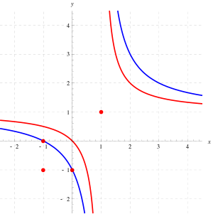
Main articles: Ising model and Potts modelAlong the hyperbola defined by (x − 1)(y − 1) = 2, the Tutte polynomial specialises to the partition function of the Ising model studied in statistical physics. More generally, along the hyperbolae Hq defined by (x − 1)(y − 1) = q for any positive integer q, the Tutte polynomial specialises to the partition function of the q-state Potts model. Various physical quantities analysed in the framework of the Potts model translate to specific parts of the Hq.
Correspondences between the Potts model and the Tutte plane [8] Potts model Tutte polynomial Ferromagnetism Positive branch of Hq Antiferromagnetism Negative branch of Hq with y > 0 High temperature Asymptote of Hq to y = 1 Low temperature ferromagnetic Positive branch of Hq asymptotic to x = 1 Zero temperature antiferromagnetic Graph q-colouring, i.e., x = 1 − q,y = 0 Flow polynomial
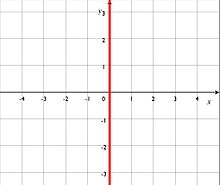
Main article: Nowhere-zero flowAt x = 0, the Tutte polynomial specialises to the flow polynomial studied in combinatorics. For a connected and undirected graph G and integer k, a nowhere-zero k-flow is an assignment of “flow” values
 to the edges of an arbitrary orientation of G such that the total flow entering and leaving each vertex is congruent modulo k. The flow polynomial CG(k) denotes the number of nowhere-zero k-flows. This value is intimately connected with the chromatic polynomial, in fact, if G is a planar graph, the chromatic polynomial of G is equivalent to the flow polynomial of its dual graph G * in the sense that
- Theorem (Tutte): C(G,k) = k − 1χ(G * ,k).
The connection to the Tutte polynomial is given by
- C(G,k) = ( − 1)m − n + 1T(0,1 − k).
Reliability polynomial
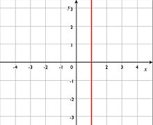
Main article: Connectivity (graph theory)At x = 1, the Tutte polynomial specialises to the all-terminal reliability polynomial studied in network theory. For a connected graph G remove every edge with probability p; this models a network subject to random edge failures. Then the reliability polynomial is a function R(G,p), a polynomial in p, that gives the probability that every pair of vertices in G remains connected after the edges fail. The connection to the Tutte polynomial is given by
Dichromatic polynomial
Tutte also defined a closer 2-variable generalization of the chromatic polynomial, the dichromatic polynomial of a graph. This is
where c(A) is the number of connected components of the spanning subgraph (V,A). This is related to the corank-nullity polynomial by
where c is the number of components of G. The dichromatic polynomial does not generalize to matroids because c is not a matroid property: different graphs with the same matroid can have different numbers of components.
Algorithms
Deletion–contraction
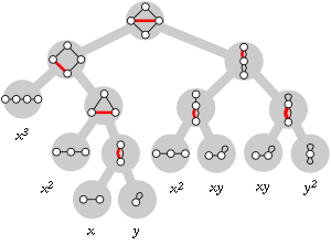 The deletion–contraction algorithm applied to the diamond graph. Red edges are deleted in the left child and contracted in the right child. The resulting polynomial is the sum of the monomials at the leaves, x3 + 2x2 + y2 + 2xy + x + y. Based on Welsh & Merino (2000).
The deletion–contraction recurrence for the Tutte polynomial,
- T(G;x,y) = T(G − e;x,y) + T(G / e;x,y) (e not a loop nor a bridge)
immediately yields a recursive algorithm for computing it: choose any such edge e and repeatedly apply the formula until all edges are either loops or bridges; the resulting base cases at the bottom of the evaluation are easy to compute.
Within a polynomial factor, the running time t of this algorithm can be expressed in terms of the number of vertices n and the number of edges m of the graph,
- t(n + m) = t(n + m − 1) + t(n + m − 2),
a recurrence relation that scales as the Fibonacci numbers with solution t(n + m) = ((1 + √5) / 2)n + m = O(1.6180n + m).[9] The analysis can be improved to within a polynomial factor of the number τ(G) of spanning trees of the input graph.[10] For sparse graphs with m = O(n) this running time is O(exp(n)). For regular graphs of degree k, the number of spanning trees can be bounded by
- τ(G) = O((νk)nn − 1log n), where νk = (k − 1)k − 1 / (k2 − 2k)k / 2 − 1
so the deletion–contraction algorithm runs within a polynomial factor of this bound. For example, for k = 5, the base of the exponent ν5 is around 4.4066.[11]
In practice, graph isomorphism testing is used to avoid some recursive calls. This approach works well for graphs that are quite sparse and exhibit many symmetries; the performance of the algorithm depends on the heuristic used to pick the edge e.[12]
Gaussian elimination
In some restricted instances, the Tutte polynomial can be computed in polynomial time, ultimately because Gaussian elimination efficiently computes the matrix operations determinant and Pfaffian. These algorithms are themselves important results from algebraic graph theory and statistical mechanics.
TG(1,1) equals the number τ(G) of spanning trees of a connected graph. This is computable in polynomial time as the determinant of a maximal principal submatrix of the Laplacian matrix of G, an early result in algebraic graph theory known as Kirchhoff’s Matrix–Tree theorem. Likewise, the dimension of the bicycle space at TG( − 1, − 1) can be computed in polynomial time by Gaussian elimination.
For planar graphs, the partition function of the Ising model, i.e., the Tutte polynomial at the hyperbola (x − 1)(y − 1) = 2, can be expressed as a Pfaffian and computed efficiently via the FKT algorithm. This idea was developed by Fisher, Kasteleyn, and Temperley to compute for the number of dimer covers of a planar lattice model.
Markov chain Monte Carlo
Using a Markov chain Monte Carlo method, the Tutte polynomial can be arbitrarily well approximated along the positive branch of H2, equivalently, the partition function of the ferromagnetic Ising model. This exploits the close connection between the Ising model and the problem of counting matchings in a graph. The idea behind this celebrated result of Jerrum and Sinclair[13] is to set up a Markov chain whose states are the matchings of the input graph. The transitions are defined by choosing edges at random and modifying the matching accordingly. The resulting Markov chain is rapidly mixing and leads to “sufficiently random” matchings, which can be used to recover the partition function using random sampling. The resulting algorithm is a fully polynomial-time randomized approximation scheme (fpras).
Computational complexity
Several computational problems are associated with the Tutte polynomial. The most straightforward one is
- Input
- A graph G
- Output
- The coefficients of TG
Especially, the output allows evaluating TG at ( − 2,0), equivalent to counting the number of 3-colourings of G This latter question is #P-complete even restricted to the family of planar graphs, so the problem of computing the coefficients of the Tutte polynomial for a given graph is #P-hard even for planar graphs.
Much more attention has been given to the family of problems called Tutte(x,y) defined for every rational pair (x,y):
- Input
- A graph G
- Output
- The value of TG(x,y)
The hardness of these problems varies with the coordinates (x,y).
Exact computation
If both x and y are nonnegative integers, the problem Tutte(x,y) belongs to #P. For general integer pairs, the Tutte polynomial contains negative terms, which places the problem in the complexity class GapP, the closure under subtraction of #P. To accommodate rational coordinates (x,y), one can define a rational analogue of #P.[14]
The computational complexity of exactly computing Tutte(x,y) is completely understood for
 . The problem is #P-hard unless (x − 1)(y − 1) = 1 or (x,y) is one of the points (1, 1), (-1, -1), (0, -1), (-1, 0), (i, -i), (-i, i), (j, j2), (j2, j) where j = e2πi / 3, in which cases it is computable in polynomial time.[15] If the problem is restricted to the class of planar graphs, the points on the hyperbola defined by (x − 1)(y − 1) = 2 become polynomial-time computable, but all other points remain #P-hard. This result contains several notable special cases. For example, the problem of computing the partition function of the Ising model is #P-hard in general, even though celebrated algorithms of Onsager and Fisher solve it for planar lattices. Also, the Jones polynomial is #P-hard to compute. Finally, computing the number of four-colourings of a planar graph is #P-complete, even though the decision problem is trivial by the four color theorem. In contrast, it is easy to see that counting the number of three-colourings for planar graphs is #P-complete because the decision problem is known to be NP-complete.
Approximation
The question which points admit a good approximation algorithm has been very well studied. Apart from the points already in P, the only approximation algorithm known for Tutte(x,y) is Jerrum and Sinclair’s FPRAS, which works for points on the “Ising” hyperbola (x − 1)(y − 1) = 2 for y > 0. If the input graphs are restricted to dense instances, with degree Ω(n), there is an FPRAS if x ≥ 1, y ≥ 1.[16]
Even though the situation is not as well understood as for exact computation, large areas of the plane are known to be hard to approximate.[14]
See also
Bollobás–Riordan polynomial
Notes
- ^ Chap. 10 in Bollobás (1998), chap. 13 in Biggs (1993), chap. 15 in Godsil & Royle (2004).
- ^ a b Tutte (2004)
- ^ Welsh
- ^ See Farr (2007)
- ^ Farr (2007)
- ^ Las Vergnas (1980).
- ^ Korn & Pak (2004), see also Korn & Pak (2003) for combinatorial interpretations of many other points
- ^ Welsh & Merino (2000)
- ^ Wilf (1986)
- ^ Sekine, Imai & Tani (1995)
- ^ Chung & Yau (1999), following Björklund et al. (2008)
- ^ Sekine, Imai & Tani (1995), Imai (2000), Haggard, Pierce & Royle (2008)
- ^ Jerrum & Sinclair (1993)
- ^ a b Goldberg & Jerrum (2008)
- ^ Jaeger, Vertigan & Welsh (1990)
- ^ x ≥ 1, y = 1 is given by Annan (1994). x ≥ 1, y > 1 is given by Alon, Frieze & Welsh (2006)
References
- Alon, N.; Frieze, A.; Welsh, D. J. A. (1995), "Polynomial time randomized approximation schemes for Tutte-Gröthendieck invariants: The dense case", Random Structures and Algorithms 6 (4): 459–478, doi:10.1002/rsa.3240060409
- Annan, J. D. (1994), "A randomised approximation algorithm for counting the number of forests in dense graphs", Combin. Prob. Comput. 3: 273–283, doi:10.1017/S0963548300001188
- Biggs, Norman (1993), Algebraic Graph Theory (2nd ed.), Cambridge: Cambridge University Press, ISBN 0-521-45897-8
- Bollobás, Béla (1998), Modern Graph Theory, Berlin, New York: Springer-Verlag, ISBN 978-0-387-98491-9
- Henry H. Crapo (1969), The Tutte polynomial. Aequationes Mathematicae, volume 3, pp. 211–229.
- Farr, G. E. (2007), "Tutte-Whitney polynomials: some history and generalizations", in Grimmett, G. R.; McDiarmid, C. J. H., Combinatorics, Complexity and Chance: A Tribute to Dominic Welsh,, Oxford University Press, pp. 28–52.
- Godsil, Chris; Royle, Gordon (2004), Algebraic Graph Theory, Berlin, New York: Springer-Verlag, ISBN 978-0-387-95220-8
- Goldberg, L.A.; Jerrum, M. (2008), "Inapproximability of the Tutte polynomial", Information and Computation 206: 908, doi:10.1016/j.ic.2008.04.003
- Jaeger, F.; Vertigan, D. L.; Welsh, D. J. A. (1990), "On the computational complexity of the Jones and Tutte polynomials", Mathematical Proceedings of the Cambridge Philosophical Society 108: 35–53, doi:10.1017/S0305004100068936
- Jerrum, M.; Sinclair, A. (1993), "Polynomial-time approximation algorithms for the Ising model", SIAM J. Comput. 22: 1087–1116, doi:10.1137/0222066
- Korn, M.; Pak, I. (2003), "Combinatorial evaluations of the Tutte polynomial", Preprint
- Korn, M.; Pak, I. (2004), "Tilings of rectangles with T-tetrominoes", Theor. Comp. Science 319: 3–27, doi:10.1016/j.tcs.2004.02.023
- Las Vergnas, Michel (1980), "Convexity in oriented matroids", Journal of Combinatorial Theory, Series B 29 (2): 231–243, doi:10.1016/0095-8956(80)90082-9, MR586435.
- Tutte, W. T. (2004), "Graph-polynomials", Advances in Applied Mathematics 32: 5–9, doi:10.1016/S0196-8858(03)00041-1
- Welsh, D. J. A.; Merino, C. (March 2000), "The Potts model and the Tutte polynomial", Journal of Mathematical Physics 41 (3)
- D.J.A. Welsh (1976), Matroid Theory. London: Academic Press.
- W.T. Tutte (1984), Graph Theory. Reading, Mass.: Addison–Wesley.
External links
- Weisstein, Eric W., "Tutte polynomial" from MathWorld.
- PlanetMath Chromatic polynomial
- Steven R. Pagano: Matroids and Signed Graphs
- Sandra Kingan: Matroid theory. Lots of links.
- Code for computing Tutte, Chromatic and Flow Polynomials by Gary Haggard, David J. Pearce and Gordon Royle: [1]
Categories:- Computational problems
- Duality theories
- Matroid theory
- Polynomials
- Graph invariants
Wikimedia Foundation. 2010.

