Contact mechanics

Continuum mechanics
Laws Conservation of mass Conservation of momentum Conservation of energy Entropy inequality
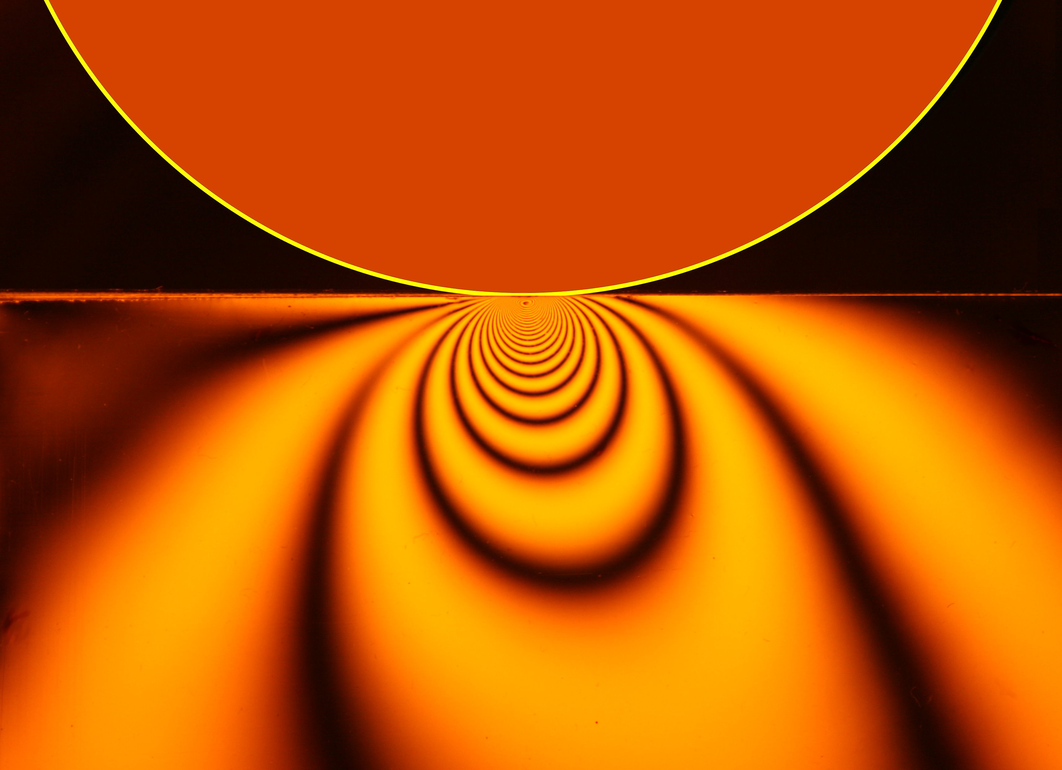
Solid mechanics Solids Stress · Deformation Compatibility Finite strain · Infinitesimal strain Elasticity (linear) · Plasticity Bending · Hooke's law Failure theory Fracture mechanics Frictionless/Frictional Contact mechanics
Fluid mechanics Fluids Fluid statics · Fluid dynamics Surface tension Navier–Stokes equations Viscosity: Newtonian, Non-Newtonian
Rheology Viscoelasticity Smart fluids: Magnetorheological Electrorheological Ferrofluids Rheometry · Rheometer
Scientists Bernoulli · Cauchy · Hooke Navier · Newton · Stokes · Jamal Nazrul Islam · Fazle Hussain
v · d · e

Stresses in a contact area loaded simultaneously with a normal and a tangential force. Stresses were made visible using photoelasticity.

Contact mechanics is the study of the deformation of solids that touch each other at one or more points.^[1][2] The physical and mathematical formulation of the subject is built upon the mechanics of materials and continuum mechanics and focuses on computations involving elastic, viscoelastic, and plastic bodies in static or dynamic contact. Central aspects in contact mechanics are the pressures and adhesion acting perpendicular to the contacting bodies' surfaces, the normal direction, and the frictional stresses acting tangentially between the surfaces. This page focuses mainly on the normal direction, i.e. on frictionless contact mechanics. Frictional contact mechanics is discussed separately.

Contact mechanics is foundational to the field of mechanical engineering; it provides necessary information for the safe and energy efficient design of technical systems and for the study of tribology and indentation hardness. Principles of contacts mechanics can be applied in areas such as locomotive wheel-rail contact, coupling devices, braking systems, tires, bearings, combustion engines, mechanical linkages, gasket seals, metalworking, metal forming, ultrasonic welding, electrical contacts, and many others. Current challenges faced in the field may include stress analysis of contact and coupling members and the influence of lubrication and material design on friction and wear. Applications of contact mechanics further extend into the micro- and nanotechnological realm.

The original work in contact mechanics dates back to 1882 with the publication of the paper "On the contact of elastic solids"^[3] ("Ueber die Berührung fester elastischer Körper") by Heinrich Hertz. Hertz was attempting to understand how the optical properties of multiple, stacked lenses might change with the force holding them together. Hertzian contact stress refers to the localized stresses that develop as two curved surfaces come in contact and deform slightly under the imposed loads. This amount of deformation is dependent on the modulus of elasticity of the material in contact. It gives the contact stress as a function of the normal contact force, the radii of curvature of both bodies and the modulus of elasticity of both bodies. Hertzian contact stress forms the foundation for the equations for load bearing capabilities and fatigue life in bearings, gears, and any other bodies where two surfaces are in contact.

History

When a sphere is pressed against an elastic material, the contact area increases.

Classical contact mechanics is most notably associated with Heinrich Hertz.^[4] In 1882 Hertz solved the problem involving contact between two elastic bodies with curved surfaces. This still-relevant classical solution provides a foundation for modern problems in contact mechanics. For example, in mechanical engineering and tribology, Hertzian contact stress, is a description of the stress within mating parts. In general, the Hertzian contact stress usually refers to the stress close to the area of contact between two spheres of different radii.

It was not until nearly one hundred years later that Johnson, Kendall, and Roberts found a similar solution for the case of adhesive contact.^[5] This theory was rejected by Boris Derjaguin and co-workers^[6] who proposed a different theory of adhesion^[7] in the 1970s. The Derjaguin model came to be known as the DMT (after Derjaguin, Muller and Toporov) model,^[7] and the Johnson et al. model came to be known as the JKR (after Johnson, Kendall and Roberts) model for adhesive elastic contact. This rejection proved to be instrumental in the development of the Tabor^[8] and later Maugis^[6][9] parameters that quantify which contact model (of the JKR and DMT models) represent adhesive contact better for specific materials.

Further advancement in the field of contact mechanics in the mid-twentieth century may be attributed to names such as Bowden and Tabor. Bowden and Tabor were the first to emphasize the importance of surface roughness for bodies in contact.^[10][11] Through investigation of the surface roughness, the true contact area between friction partners is found to be less than the apparent contact area. Such understanding also drastically changed the direction of undertakings in tribology. The works of Bowden and Tabor yielded several theories in contact mechanics of rough surfaces.

The contributions of Archard (1957)^[12] must also be mentioned in discussion of pioneering works in this field. Archard concluded that, even for rough elastic surfaces, the contact area is approximately proportional to the normal force. Further important insights along these lines were provided by Greenwood and Williamson (1966),^[13] Bush (1975),^[14] and Persson (2002).^[15] The main findings of these works were that the true contact surface in rough materials is generally proportional to the normal force, while the parameters of individual micro-contacts (i.e. pressure, size of the micro-contact) are only weakly dependent upon the load.

Classical solutions for non-adhesive elastic contact

The theory of contact between elastic bodies can be used to find contact areas and indentation depths for simple geometries. Some commonly used solutions are listed below. The theory used to compute these solutions is discussed later in the article.

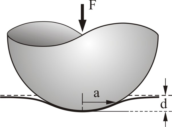
Contact between a sphere and an elastic half-space

Contact between a sphere and an elastic half-space

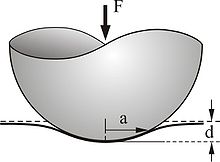
An elastic sphere of radius R indents an elastic half-space to depth d, and thus creates a contact area of radius $a=\sqrt{Rd}$. The applied force F is related to the displacement d by

$F=\tfrac{4}{3}E^*R^{1/2}d^{3/2}$

where

$\frac{1}{E^*}=\frac{1-\nu^2_1}{E_1}+\frac{1-\nu^2_2}{E_2}$

and E₁,E₂ are the elastic moduli and ν₁,ν₂ the Poisson's ratios associated with each body.

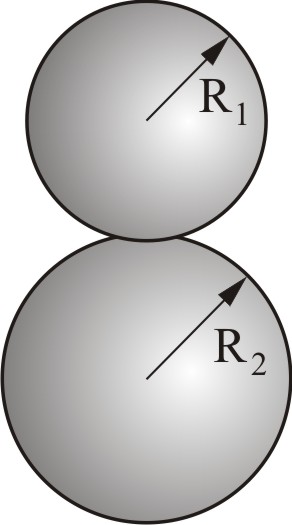
Contact between two spheres

Contact between two spheres

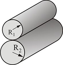
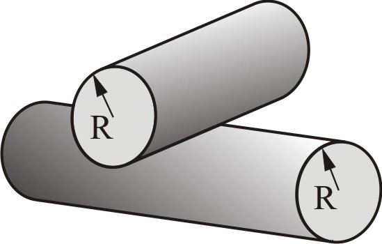
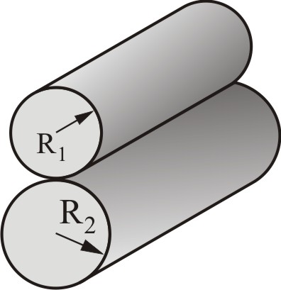
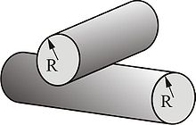Contact between two crossed cylinders of equal radius

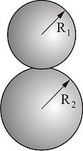
For contact between two spheres of radii R₁ and R₂, the area of contact is a circle of radius a. The distribution of normal traction in the contact area as a function of distance from the center of the circle is^[1]

$p(r) = p_0\left(1-\frac{r^2}{a^2}\right)^{1/2}$

where p₀ is the maximum contact pressure given by

$p_0 = \cfrac{3F}{2\pi a^2} = \cfrac{1}{\pi}\left(\cfrac{6F{E^*}^2}{R^2}\right)^{1/3}$

where the effective radius R is defined as

$\frac{1}{R} = \frac{1}{R_1}+\frac{1}{R_2}$

The area of contact is related to the applied load F by the equation

$a^3 = \cfrac{3 F R}{4 E^*}$

The depth of indentation d is related to the maximum contact pressure by

$d = \cfrac{a^2}{R} = \left(\cfrac{9F^2}{16R{E^*}^2}\right)^{1/3}$

The maximum shear stress occurs in the interior at $z\approx 0.49a$ for ν = 0.33.

Contact between two crossed cylinders of equal radius R

This is equivalent to contact between a sphere of radius R and a plane (see above).

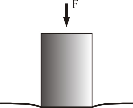
Contact between a rigid cylinder and an elastic half-space

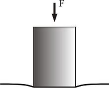Contact between a rigid cylindrical indenter and an elastic half-space

If a rigid cylinder is pressed into an elastic half-space, it creates a pressure distribution described by^[16]

$p(r)=p_0\left(1-\frac{r^2}{a^2}\right)^{-1/2}$

where a is the radius of the cylinder and

$p_0=\frac{1}{\pi}E^*\frac{d}{a}$

The relationship between the indentation depth and the normal force is given by

$F=2aE^*d\,$

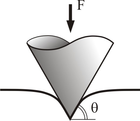
Contact between a rigid conical indenter and an elastic half-space

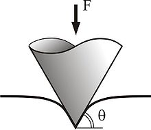Contact between a rigid conical indenter and an elastic half-space

In the case of indentation of an elastic half-space using a rigid conical indenter, the indentation depth and contact radius are related by^[16]

$d=\frac{\pi}{2}a\tan\theta$

with θ defined as the angle between the plane and the side surface of the cone. The pressure distribution takes on the form

$p(r)=-\frac{Ed}{\pi a\left(1-\nu^2\right)}\ln\left(\frac{a}{r}+\sqrt{\left(\frac{a}{r}\right)^2-1}\right)$

The stress has a logarithmic singularity on the tip of the cone. The total force is

$F_N=\frac{2}{\pi}E^*\frac{d^2}{\tan \theta}$

Contact between two cylinders with parallel axes

Contact between two cylinders with parallel axes

In contact between two cylinders with parallel axes, the force is linearly proportional to the indentation depth:

$F=\frac{\pi}{4}E^*Ld$

The radii of curvature are entirely absent from this relationship. The contact radius is described through the usual relationship

$a=\sqrt{Rd}$

with

$\frac{1}{R}=\frac{1}{R_1}+\frac{1}{R_2}$

as in contact between two spheres. The maximum pressure is equal to

$p_0=\left(\frac{E^*F}{\pi LR}\right)^{1/2}$

Hertzian theory of non-adhesive elastic contact

The classical theory of contact focused primarily on non-adhesive contact where no tension force is allowed to occur within the contact area, i.e., contacting bodies can be separated without adhesion forces. Several analytical and numerical approaches have been used to solve contact problems that satisfy the no-adhesion condition. Complex forces and moments are transmitted between the bodies where they touch, so problems in contact mechanics can become quite sophisticated. In addition, the contact stresses are usually a nonlinear function of the deformation. To simplify the solution procedure, a frame of reference is usually defined in which the objects (possibly in motion relative to one another) are static. They interact through surface tractions (or pressures/stresses) at their interface.

As an example, consider two objects which meet at some surface S in the (x,y)-plane with the z-axis assumed normal to the surface. One of the bodies will experience a normally-directed pressure distribution p_z = p(x,y) = q_z(x,y) and in-plane surface traction distributions q_x = q_x(x,y) and q_y = q_y(x,y) over the region S. In terms of a Newtonian force balance, the forces:

$P_z = \int_S p(x,y)~ \mathrm{d}A ~;~~ Q_x = \int_S q_x(x,y)~ \mathrm{d}A ~;~~ Q_y = \int_S q_y(x,y)~ \mathrm{d}A$

must be equal and opposite to the forces established in the other body. The moments corresponding to these forces:

$M_x = \int_S y~p(x,y)~ \mathrm{d}A ~;~~ M_y = \int_S x~p(x,y)~ \mathrm{d}A ~;~~ M_z = \int_S [x~q_y(x,y) - y~q_x(x,y)]~ \mathrm{d}A$

are also required to cancel between bodies so that they are kinematically immobile.

Assumptions in Hertzian theory

The following assumptions are made in determining the solutions of Hertzian contact problems:

• the strains are small and within the elastic limit,
• each body can be considered an elastic half-space, i.e., the area of contact is much smaller than the characteristic radius of the body,
• the surfaces are continuous and non-conforming, and
• the surfaces are frictionless.

Additional complications arise when some or all these assumptions are violated and such contact problems are usually called non-Hertzian.

Analytical solution techniques

Contact between two spheres.

Analytical solution methods for non-adhesive contact problem can be classified into two types based on the geometry of the area of contact.^[17] A conforming contact is one in which the two bodies touch at multiple points before any deformation takes place (i.e., they just "fit together"). A non-conforming contact is one in which the shapes of the bodies are dissimilar enough that, under zero load, they only touch at a point (or possibly along a line). In the non-conforming case, the contact area is small compared to the sizes of the objects and the stresses are highly concentrated in this area. Such a contact is called concentrated, otherwise it is called diversified.

A common approach in linear elasticity is to superpose a number of solutions each of which corresponds to a point load acting over the area of contact. For example, in the case of loading of a half-plane, the Flamant solution is often used as a starting point and then generalized to various shapes of the area of contact. The force and moment balances between the two bodies in contact act as additional constraints to the solution.

Point contact on a (2D) half-plane

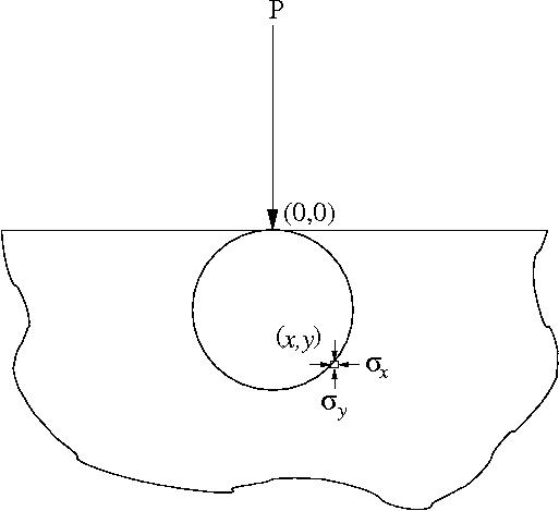
Main article: Flamant solution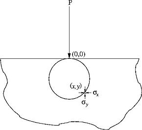

Schematic of the loading on a plane by force P at a point (0,0).

A starting point for solving contact problems is to understand the effect of a "point-load" applied to an isotropic, homogeneous, and linear elastic half-plane, shown in the figure to the right. The problem may be either be plane stress or plane strain. This is a boundary value problem of linear elasticity subject to the traction boundary conditions:

$\sigma_{xz} (x,0)=0 ~;~~ \sigma_z (x,z)=-P\delta (x,z)$

where δ(x,z) is the Dirac delta function. The boundary conditions state that are no shear stresses on the surface and a singular normal force P is applied at (0,0). Applying these conditions to the governing equations of elasticity produces the result

$\begin{align} \sigma_{xx} & =-\frac{2P}{\pi}\frac{x^2z}{(x^2+z^2)^2} ~;~~ \sigma_{zz} =-\frac{2P}{\pi}\frac{z^3}{(x^2+z^2)^2} \\ \sigma_{xz} & =-\frac{2P}{\pi}\frac{xz^2}{(x^2+z^2)^2} \end{align}$

for some point, (x,y), in the half-plane. The circle shown in the figure indicates a surface on which the maximum shear stress is constant. From this stress field, the strain components and thus the displacements of all material points may be determined.

Line contact on a (2D) half-plane

Normal loading over a region (a,b)

Suppose, rather than a point load P, a distributed load p(x) is applied to the surface instead, over the range a < x < b. The principle of linear superposition can be applied to determine the resulting stress field as the solution to the integral equations:

$\begin{align} \sigma_{xx} & =-\frac{2z}{\pi}\int_a^b\frac{p(x')(x-x')^2\, dx'}{[(x-x')^2+z^2]^2} ~;~~ \sigma_{zz} =-\frac{2z^3}{\pi}\int_a^b\frac{p(x')(x-x')^2\, dx'}{[(x-x')^2+z^2]^2} \\ \sigma_{xz} & =-\frac{2z^2}{\pi}\int_a^b\frac{p(x')(x-x')\, dx'}{[(x-x')^2+z^2]^2} \end{align}$

Shear loading over a region (a,b)

The same principle applies for loading on the surface in the plane of the surface. These kinds of tractions would tend to arise as a result of friction. The solution is similar the above (for both singular loads Q and distributed loads q(x)) but altered slightly:

$\begin{align} \sigma_{xx} & =-\frac{2}{\pi}\int_a^b\frac{q(x')(x-x')^3\, dx'}{[(x-x')^2+z^2]^2} ~;~~ \sigma_{zz} =-\frac{2z^2}{\pi}\int_a^b\frac{q(x')(x-x')\, dx'}{[(x-x')^2+z^2]^2} \\ \sigma_{xz} & =-\frac{2z}{\pi}\int_a^b\frac{q(x')(x-x')^2\, dx'}{[(x-x')^2+z^2]^2} \end{align}$

These results may themselves be superposed onto those given above for normal loading to deal with more complex loads.

Point contact on a (3D) half-space

Analogously to the Flamant solution for the 2D half-plane, fundamental solutions are known for the linearly elastic 3D half-space as well. These were found by Boussinesq for a concentrated normal load and by Cerutti for a tangential load. See the section on this in Linear elasticity.

Numerical solution techniques

Distinctions between conforming and non-conforming contact do not have to be made when numerical solution schemes are employed to solve contact problems. These methods do not rely on further assumptions within the solution process since they base solely on the general formulation of the underlying equations ^{[18] [19] [20] [21]} .^[22] Besides the standard equations describing the deformation and motion of bodies two additional inequalities can be formulated. The first simply restricts the motion and deformation of the bodies by the assumption that no penetration can occur. Hence the gap g_N between two bodies can only be positive or zero

$g_N \ge 0$

where g_N = 0 denotes contact. The second assumption in contact mechanics is related to the fact, that no tension force is allowed to occur within the contact area (contacting bodies can be lifted up without adhesion forces). This leads to an inequality which the stresses have to obey at the contact interface. It is formulated for the contact pressure $p_N = \mathbf{t} \cdot \mathbf{n}$

$p_N \le 0 \,.$

Since for contact, g_N = 0, the contact pressure is always negative, p_N < 0, and further for non contact the gap is open, g_N > 0, and the contact pressure is zero, p_N = 0, the so called Kuhn–Tucker form of the contact constraints can be written as

$g_N \ge 0\,, \quad p_N \le 0\,, \quad p_N\,g_N = 0\,.$

These conditions are valid in a general way. The mathematical formulation of the gap depends upon the kinematics of the underlying theory of the solid (e.g., linear or nonlinear solid in two- or three dimensions, beam or shell model).

Non-adhesive contact between rough surfaces

When two bodies with rough surfaces are pressed into each other, the true contact area A is much smaller than the apparent contact area A₀. In contact between a "random rough" surface and an elastic half-space, the true contact area is related to the normal force F by^{[1][23][24][25]}

$A=\frac{\kappa}{E^*h'}F$

with h' equal to the root mean square (also known as the quadratic mean) of the surface slope and $\kappa \approx2$ . The median pressure in the true contact surface

$p_{\mathrm{av}} =\frac{F}{A}\approx\frac{1}{2}E^*h'$

can be reasonably estimated as half of the effective elastic modulus E ^* multiplied with the root mean square of the surface slope h' .

For the situation where the asperities on the two surfaces have a Gaussian height distribution and the peaks can be assumed to be spherical,^[23] the average contact pressure is sufficient to cause yield when $p_{\mathrm{av}} = 1.1\sigma_y \approx 0.39 \sigma_0$ where σ_y is the uniaxial yield stress and σ₀ is the indentation hardness.^[1] Greenwood and Williamson^[23] defined a dimensionless parameter Ψ called the plasticity index that could be used to determine whether contact would be elastic or plastic.

The Greenwood-Williamson model requires knowledge of two statistically dependent quantities; the standard deviation of the surface roughness and the curvature of the asperity peaks. An alternative definition of the plasticity index has been given by Mikic.^[24] Yield occurs when the pressure is greater than the uniaxial yield stress. Since the yield stress is proportional to the indentation hardness σ₀, Micic defined the plasticity index for elastic-plastic contact to be

$\Psi = \frac{E^*h'}{\sigma _0}> \tfrac{2}{3}~.$

In this definition Ψ represents the micro-roughness in a state of complete plasticity and only one statistical quantity, the rms slope, is needed which can be calculated from surface measurements. For $\Psi <\tfrac{2}{3}$, the surface behaves elastically during contact.

In both the Greenwood-Williamson and Mikic models the load is assumed to be proportional to the deformed area. Hence, whether the system behaves plastically or elastically is independent of the applied normal force.^[1]

Adhesive contact between elastic bodies

When two solid surfaces are brought into close proximity to each other they experience attractive van der Waals forces. Bradley's van der Waals model^[26] provides a means of calculating the tensile force between two rigid spheres with perfectly smooth surfaces. The Hertzian model of contact does not consider adhesion possible. However, in the late 1960s, several contradictions were observed when the Hertz theory was compared with experiments involving contact between rubber and glass spheres.

It was observed^[5] that, though Hertz theory applied at large loads, at low loads

• the area of contact was larger than that predicted by Hertz theory,
• the area of contact had a non-zero value even when the load was removed, and
• there was strong adhesion if the contacting surfaces were clean and dry.

This indicated that adhesive forces were at work. The Johnson-Kendall-Roberts (JKR) model and the Derjaguin-Muller-Toporov (DMT) models were the first to incorporate adhesion into Hertzian contact.

Bradley model of rigid contact

It is commonly assumed that the surface force between two atomic planes at a distance z from each other can be derived from the Lennard-Jones potential. With that assumption we can write

$f(z) = \cfrac{16\gamma}{3 z_0}\left[\left(\cfrac{z}{z_0}\right)^{-9} - \left(\cfrac{z}{z_0}\right)^{-3}\right]$

where f is the force (positive in compression), 2γ is the is the total surface energy of both surfaces per unit area, and z₀ is the equilibrium separation of the two atomic planes.

The Bradley model applied the Lennard-Jones potential to find the force of adhesion between two rigid spheres. The total force between the spheres is found to be

$F_a = \cfrac{16\gamma\pi R}{3}\left[\cfrac{1}{4}\left(\cfrac{z}{z_0}\right)^{-8} - \left(\cfrac{z}{z_0}\right)^{-2}\right] ~;~~ \frac{1}{R} = \frac{1}{R_1} + \frac{1}{R_2}$

where R₁,R₂ are the radii of the two spheres.

The two spheres separate completely when the pull-off force is achieved at z = z₀ at which point

$F_a = F_c = -4\gamma\pi R \,$

Johnson-Kendall-Roberts (JKR) model of elastic contact

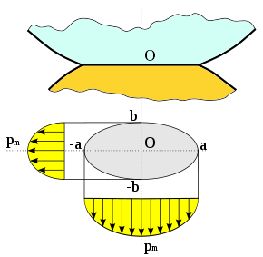
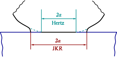Schematic of contact area for the JKR model.

To incorporate the effect of adhesion in Hertzian contact, Johnson, Kendall, and Roberts^[5] formulated the JKR theory of adhesive contact using a balance between the stored elastic energy and the loss in surface energy. The JKR model considers the effect of contact pressure and adhesion only inside the area of contact. The general solution for the pressure distribution in the contact area in the JKR model is

$p(r) = p_0\left(1 - \cfrac{r^2}{a^2}\right)^{1/2} + p_0'\left(1 - \cfrac{r^2}{a^2}\right)^{-1/2}$

Note that in the original Hertz theory, the term containing p₀' was neglected on the ground that tension could not be sustained in the contact zone. For contact between two spheres

$p_0 = \cfrac{2 a E^*}{\pi R} ~;~~ p_0' = -\left(\cfrac{4\gamma E^*}{\pi a}\right)^{1/2}$

where $a\,$ is the radius of the area of contact, F is the applied force, 2γ is the total surface energy of both surfaces per unit contact area, $R_i, E_i, \nu_i,~~i=1,2$ are the radii, Young's moduli, and Poisson's ratios of the two spheres, and

$\frac{1}{R} = \frac{1}{R_1} + \frac{1}{R_2} ~;~~ \frac{1}{E^*} = \frac{1-\nu_1^2}{E_1} + \frac{1-\nu_2^2}{E_2}$

The approach distance between the two spheres is given by

$d = \cfrac{\pi a}{2 E^*}(p_0 + 2p_0') = \cfrac{a^2}{R}$

The Hertz equation for the area of contact between two spheres, modified to take into account the surface energy, has the form

$a^3 = \cfrac{3R}{4E^*}\left(F + 6\gamma\pi R + \sqrt{12\gamma\pi R F + (6\gamma\pi R)^2}\right)$

When the surface energy is zero, γ = 0, the Hertz equation for contact between two spheres is recovered. When the applied load is zero, the contact radius is

$a^3 = \cfrac{9R^2\gamma\pi}{E^*}$

The tensile load at which the spheres are separated, i.e., a = 0, is predicted to be

$F_c = -3\gamma\pi R\,$

This force is also called the pull-off force. Note that this force is independent of the moduli of the two spheres. However, there is another possible solution for the value of a at this load. This is the critical contact area a_c, given by

$a_c^3 = \cfrac{9R^2\gamma\pi}{4E^*}$

If we define the work of adhesion as

Δγ = γ₁ + γ₂ − γ₁₂

where γ₁,γ₂ are the adhesive energies of the two surfaces and γ₁₂ is an interaction term, we can write the JKR contact radius as

$a^3 = \cfrac{3R}{4E^*}\left(F + 3\Delta\gamma\pi R + \sqrt{6\Delta\gamma\pi R F + (3\Delta\gamma\pi R)^2}\right)$

The tensile load at separation is

$F = -\cfrac{3}{2}\Delta\gamma\pi R\,$

and the critical contact radius is given by

$a_c^3 = \cfrac{9R^2\Delta\gamma\pi}{4E^*}$

The critical depth of penetration is

$d_c = \cfrac{a_c^2}{R} = \left(\cfrac{9}{4}\right)^{\tfrac{2}{3}}(\Delta\gamma)^{\tfrac{2}{3}}\left(\cfrac{\pi^{\tfrac{2}{3}}~R^{\tfrac{1}{3}}}{{E^*}^{\tfrac{2}{3}}}\right)$

Derjaguin-Muller-Toporov (DMT) model of elastic contact

The Derjaguin-Muller-Toporov (DMT) model^[27][28] is an alternative model for adhesive contact which assumes that the contact profile remains the same as in Hertzian contact but with additional attractive interactions outside the area of contact.

The area of contact between two spheres from DMT theory is

$a^3 = \cfrac{3R}{4E^*}\left(F + 4\gamma\pi R\right)$

and the pull-off force is

$F_c = -4\gamma\pi R\,$

When the pull-off force is achieved the contact area becomes zero and there is no singularity in the contact stresses at the edge of the contact area.

In terms of the work of adhesion Δγ

$a^3 = \cfrac{3R}{4E^*}\left(F + 2\Delta\gamma\pi R\right)$

and

$F_c = -2\Delta\gamma\pi R\,$

Tabor coefficient

In 1977, Tabor^[29] showed that the apparent contradiction between the JKR and DMT theories could be resolved by noting that the two theories were the extreme limits of a single theory parametrized by the Tabor coefficient (μ) defined as

$\mu := \cfrac{d_c}{z_0} \approx \left[\cfrac{R(\Delta\gamma)^2}{{E^*}^2 z_0^3}\right]^{1/3}$

where z₀ is the equilibrium separation between the two surfaces in contact. The JKR theory applies to large, compliant spheres for which μ is large. The DMT theory applies for small, stiff spheres with small values of μ.

Maugis-Dugdale model of elastic contact

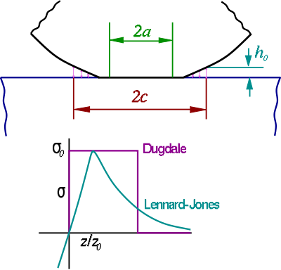Schematic of contact area for the Maugis-Dugdale model.

Further improvement to the Tabor idea was provided by Maugis^[9] who represented the surface force in terms of a Dugdale cohesive zone approximation such that the work of adhesion is given by

$\Delta\gamma = \sigma_0~h_0$

where σ₀ is the maximum force predicted by the Lennard-Jones potential and h₀ is the maximum separation obtained by matching the areas under the Dugdale and Lennard-Jones curves (see adjacent figure). This means that the attractive force is constant for $z_0 \le z \le z_0 + h_0$. There is not further penetration in compression. Perfect contact occurs in an area of radius a and adhesive forces of magnitude σ₀ extend to an area of radius c > a. In the region a < r < c, the two surfaces are separated by a distance h(r) with h(a) = 0 and h(c) = h₀. The ratio m is defined as

$m := \cfrac{c}{a}$.

In the Maugis-Dugdale theory,^[30] the surface traction distribution is divided into two parts - one due to the Hertz contact pressure and the other from the Dugdale adhesive stress. Hertz contact is assumed in the region − a < r < a. The contribution to the surface traction from the Hertz pressure is given by

$p^H(r) = \left(\cfrac{3F^H}{2\pi a^2}\right)\left(1 - \cfrac{r^2}{a^2}\right)^{1/2}$

where the Hertz contact force F^H is given by

$F^H = \cfrac{4E^*a^3}{3R}$

The penetration due to elastic compression is

$d^H = \cfrac{a^2}{R}$

The vertical displacement at r = c is

$u^H(c) = \cfrac{1}{\pi R} \left[a^2(2 - m^2)\sin^{-1}\left(\cfrac{1}{m}\right) + a^2\sqrt{m^2-1}\right]$

and the separation between the two surfaces at r = c is

$h^H(c) = \cfrac{c^2}{2R} - d^H + u^H(c)$

The surface traction distribution due to the adhesive Dugdale stress is

$p^D(r) = \begin{cases} -\cfrac{\sigma_0}{\pi}\cos^{-1}\left[\cfrac{2-m^2-\cfrac{r^2}{a^2}}{m^2\left(1-\cfrac{r^2}{m^2a^2}\right)}\right] & \quad \mathrm{for} \quad r \le a\\ -\sigma_0 & \quad \mathrm{for} \quad a \le r \le c \end{cases}$

The total adhesive force is then given by

$F^D = -2\sigma_0 m^2a^2\left[\cos^{-1}\left(\cfrac{1}{m}\right) + \frac{1}{m^2}\sqrt{m^2 - 1}\right]$

The compression due to Dugdale adhesion is

$d^D = -\left(\cfrac{2\sigma_0 a}{E^*}\right)\sqrt{m^2-1}$

and the gap at r = c is

$h^D(c) = \left(\cfrac{4\sigma_0 a}{\pi E^*}\right)\left[\sqrt{m^2-1}\cos^{-1}\left(\cfrac{1}{m}\right) + 1-m\right]$

The net traction on the contact area is then given by p(r) = p^H(r) + p^D(r) and the net contact force is F = F^H + F^D. When h(c) = h^H(c) + h^D(c) = h₀ the adhesive traction drops to zero.

Non-dimensionalized values of a,c,F,d are introduced at this stage that are defied as

$\bar{a} = \alpha a ~;~~ \bar{c} := \alpha c ~;~~ \bar{d} := \alpha^2 R d ~;~~ \alpha := \left(\cfrac{4E^*}{3\pi\Delta\gamma R^2}\right)^{1/3} ~;~~ \bar{A} := \pi c^2 ~;~~ \bar{F} = \cfrac{F}{\pi\Delta\gamma R}$

In addition, Maugis proposed a parameter λ which is equivalent to the Tabor coefficient. This parameter is defined as

$\lambda := 1.16\mu = \sigma_0\left(\cfrac{9R}{2\pi\Delta\gamma{E^*}^2}\right)^{1/3}$

Then the net contact force may be expressed as

$\bar{F} = \bar{a}^3 - \cfrac{4}{3}~\lambda \bar{a}^2\left[\sqrt{m^2 -1} + m^2 \sec^{-1} m\right]$

and the elastic compression as

$\bar{d} = \bar{a}^2 - \cfrac{4}{3}~\lambda \bar{a}\sqrt{m^2-1}$

The equation for the cohesive gap between the two bodies takes the form

$\cfrac{\lambda \bar{a}^2}{2}\left[(m^2-2)\sec^{-1} m + \sqrt{m^2-1}\right] + \cfrac{4\lambda\bar{a}}{3}\left[\sqrt{m^2-1}\sec^{-1} m - m + 1\right] = 1$

This equation can be solved to obtain values of c for various values of a and λ. For large values of λ, $m \rightarrow 1$ and the JKR model is obtained. For small values of λ the DMT model is retrieved.

Carpick-Ogletree-Salmeron (COS) model

The Maugis-Dugdale model can only be solved iteratively if the value of λ is not known a-priori. The Carpick-Ogletree-Salmeron approximate solution ^[31] simplifies the process by using the following relation to determine the contact radius a:

$a = a_0(\beta) \left(\cfrac{\beta + \sqrt{1 - F/F_c(\beta)}}{1 + \beta}\right)^{2/3}$

where a₀ is the contact area at zero load, and β is a transition parameter that is related to λ by

λ = − 0.924ln(1 − 1.02β)

The case β = 1 corresponds exactly to JKR theory while β = 0 corresponds to DMT theory. For intermediate cases 0 < β < 1 the COS model corresponds closely to the Maugis-Dugdale solution for 0.1 < λ < 5.

See also

• Adhesive
• Adhesive bonding
• Adhesive dermatitis
• Adhesive surface forces
• Bearing capacity
• Bioadhesives
• Contact dynamics
• Dispersive adhesion
• Electrostatic generator
• Frictional contact mechanics
• Galling
• Goniometer
• Non-smooth mechanics
• Plastic wrap
• Shock (mechanics)
• Signorini problem
• Surface tension
• Synthetic setae
• Unilateral contact
• Wetting

References

1. ^ ^{a b c d e} Johnson, K. L, 1985, Contact mechanics, Cambridge University Press.
2. ^ Popov, Valentin L., 2010, Contact Mechanics and Friction. Physical Principles and Applications, Springer-Verlag, 362 p., ISBN 978-3-642-10802-0.
3. ^ H. Hertz, Über die berührung fester elastischer Körper (On the contact of rigid elastic solids). In: Miscellaneous Papers. Jones and Schott, Editors, J. reine und angewandte Mathematik 92, Macmillan, London (1896), p. 156 English translation: Hertz, H.
4. ^ Hertz, H. R., 1882, Ueber die Beruehrung elastischer Koerper (On Contact Between Elastic Bodies), in Gesammelte Werke (Collected Works), Vol. 1, Leipzig, Germany, 1895.
5. ^ ^{a b c} K. L. Johnson and K. Kendall and A. D. Roberts, Surface energy and the contact of elastic solids, Proc. R. Soc. London A 324 (1971) 301-313
6. ^ ^{a b} D. Maugis, Contact, Adhesion and Rupture of Elastic Solids, Springer-Verlag, Solid-State Sciences, Berlin 2000, ISBN 3-540-66113-1
7. ^ ^{a b} B. V. Derjaguin and V. M. Muller and Y. P. Toporov, Effect of contact deformations on the adhesion of particles, J. Colloid Interface Sci. 53 (1975) 314--325
8. ^ D. Tabor, The hardness of solids, J. Colloid Interface Sci. 58 (1977) 145-179
9. ^ ^{a b} D. Maugis, Adhesion of spheres: The JKR-DMT transition using a Dugdale model, J. Colloid Interface Sci. 150 (1992) 243--269
10. ^ , Bowden, FP and Tabor, D., 1939, The area of contact between stationary and between moving surfaces, Proceedings of the Royal Society of London. Series A, Mathematical and Physical Sciences, 169(938), pp. 391--413.
11. ^ Bowden, F.P. and Tabor, D., 2001, The friction and lubrication of solids, Oxford University Press.
12. ^ Archard, JF, 1957, Elastic deformation and the laws of friction, Proceedings of the Royal Society of London. Series A, Mathematical and Physical Sciences, 243(1233), pp.190--205.
13. ^ Greenwood, JA and Williamson, JBP., 1966, Contact of nominally flat surfaces, Proceedings of the Royal Society of London. Series A, Mathematical and Physical Sciences, pp. 300-319.
14. ^ Bush, AW and Gibson, RD and Thomas, TR., 1975, The elastic contact of a rough surface, Wear, 35(1), pp. 87-111.
15. ^ Persson, BNJ and Bucher, F. and Chiaia, B., 2002, Elastic contact between randomly rough surfaces: Comparison of theory with numerical results, Physical Review B, 65(18), p. 184106.
16. ^ ^{a b} Sneddon, I. N., 1965, The Relation between Load and Penetration in the Axisymmetric Boussinesq Problem for a Punch of Arbitrary Profile. Int. J. Eng. Sci. v. 3, pp. 47–57.
17. ^ Shigley, J.E., Mischke, C.R., 1989, Mechanical Engineering Design, Fifth Edition, Chapter 2, McGraw-Hill, Inc, 1989, ISBN 0-07-056899-5.
18. ^ Kalker, J.J. 1990, Three-Dimensional Elastic Bodies in Rolling Contact. (Kluwer Academic Publishers: Dordrecht).
19. ^ Wriggers, P. 2006, Computational Contact Mechanics. 2nd ed. (Springer Verlag: Heidelberg).
20. ^ Laursen, T. A., 2002, Computational Contact and Impact Mechanics: Fundamentals of Modeling Interfacial Phenomena in Nonlinear Finite Element Analysis, (Springer Verlag: New York).
21. ^ Acary V. and Brogliato B., 2008,Numerical Methods for Nonsmooth Dynamical Systems. Applications in Mechanics and Electronics. Springer Verlag, LNACM 35, Heidelberg.
22. ^ Popov, Valentin L., 2009, Kontaktmechanik und Reibung. Ein Lehr- und Anwendungsbuch von der Nanotribologie bis zur numerischen Simulation, Springer-Verlag, 328 S., ISBN 978-3-540-88836-9.
23. ^ ^{a b c} Greenwood, J. A. and Williamson, J. B. P., (1966), Contact of nominally flat surfaces, Proceedings of the Royal Society of London. Series A, Mathematical and Physical Sciences, vol. 295, pp. 300--319.
24. ^ ^{a b} Mikic, B. B., (1974), Thermal contact conductance; theoretical considerations, International Journal of Heat and Mass Transfer, 17(2), pp. 205-214.
25. ^ Hyun, S., and M.O. Robbins, 2007, Elastic contact between rough surfaces: Effect of roughness at large and small wavelengths. Trobology International, v.40, pp. 1413-1422.
26. ^ Bradley, RS., 1932, The cohesive force between solid surfaces and the surface energy of solids, Philosophical Magazine Series 7, 13(86), pp. 853--862.
27. ^ Derjaguin, BV and Muller, VM and Toporov, Y.P., 1975, Effect of contact deformations on the adhesion of particles, Journal of Colloid and Interface Science, 53(2), pp. 314-326.
28. ^ Muller, VM and Derjaguin, BV and Toporov, Y.P., 1983, On two methods of calculation of the force of sticking of an elastic sphere to a rigid plane, Colloids and Surfaces, 7(3), pp. 251-259.
29. ^ Tabor, D., 1977, Surface forces and surface interactions, Journal of Colloid and Interface Science, 58(1), pp. 2-13.
30. ^ Johnson, KL and Greenwood, JA, 1997, An adhesion map for the contact of elastic spheres, Journal of Colloid and Interface Science, 192(2), pp. 326-333.
31. ^ Carpick, R.W. and Ogletree, D.F. and Salmeron, M., 1999, A general equation for fitting contact area and friction vs load measurements, Journal of colloid and interface science, 211(2), pp. 395-400.

External links

• [1]: More about contact stresses and the evolution of bearing stress equations can be found in this publication by NASA Glenn Research Center head the NASA Bearing, Gearing and Transmission Section, Erwin Zaretsky.