Dynamical system

This article is about the general aspects of dynamical systems. For technical details, see Dynamical system (definition). For the study, see Dynamical systems theory.

"Dynamical" redirects here. For other uses, see Dynamics (disambiguation).

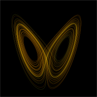The Lorenz attractor is an example of a non-linear dynamical system. Studying this system helped give rise to Chaos theory.

A dynamical system is a concept in mathematics where a fixed rule describes the time dependence of a point in a geometrical space. Examples include the mathematical models that describe the swinging of a clock pendulum, the flow of water in a pipe, and the number of fish each springtime in a lake.

At any given time a dynamical system has a state given by a set of real numbers (a vector) that can be represented by a point in an appropriate state space (a geometrical manifold). Small changes in the state of the system create small changes in the numbers. The evolution rule of the dynamical system is a fixed rule that describes what future states follow from the current state. The rule is deterministic; in other words, for a given time interval only one future state follows from the current state.

Overview

The concept of a dynamical system has its origins in Newtonian mechanics. There, as in other natural sciences and engineering disciplines, the evolution rule of dynamical systems is given implicitly by a relation that gives the state of the system only a short time into the future. (The relation is either a differential equation, difference equation or other time scale.) To determine the state for all future times requires iterating the relation many times—each advancing time a small step. The iteration procedure is referred to as solving the system or integrating the system. Once the system can be solved, given an initial point it is possible to determine all its future positions, a collection of points known as a trajectory or orbit.

Before the advent of fast computing machines, solving a dynamical system required sophisticated mathematical techniques and could be accomplished only for a small class of dynamical systems. Numerical methods implemented on electronic computing machines have simplified the task of determining the orbits of a dynamical system.

For simple dynamical systems, knowing the trajectory is often sufficient, but most dynamical systems are too complicated to be understood in terms of individual trajectories. The difficulties arise because:

• The systems studied may only be known approximately—the parameters of the system may not be known precisely or terms may be missing from the equations. The approximations used bring into question the validity or relevance of numerical solutions. To address these questions several notions of stability have been introduced in the study of dynamical systems, such as Lyapunov stability or structural stability. The stability of the dynamical system implies that there is a class of models or initial conditions for which the trajectories would be equivalent. The operation for comparing orbits to establish their equivalence changes with the different notions of stability.
• The type of trajectory may be more important than one particular trajectory. Some trajectories may be periodic, whereas others may wander through many different states of the system. Applications often require enumerating these classes or maintaining the system within one class. Classifying all possible trajectories has led to the qualitative study of dynamical systems, that is, properties that do not change under coordinate changes. Linear dynamical systems and systems that have two numbers describing a state are examples of dynamical systems where the possible classes of orbits are understood.
• The behavior of trajectories as a function of a parameter may be what is needed for an application. As a parameter is varied, the dynamical systems may have bifurcation points where the qualitative behavior of the dynamical system changes. For example, it may go from having only periodic motions to apparently erratic behavior, as in the transition to turbulence of a fluid.
• The trajectories of the system may appear erratic, as if random. In these cases it may be necessary to compute averages using one very long trajectory or many different trajectories. The averages are well defined for ergodic systems and a more detailed understanding has been worked out for hyperbolic systems. Understanding the probabilistic aspects of dynamical systems has helped establish the foundations of statistical mechanics and of chaos.

It was in the work of Poincaré that these dynamical systems themes developed.

Basic definitions

Main article: Dynamical system (definition)

A dynamical system is a manifold M called the phase (or state) space endowed with a family of smooth evolution functions Φ ^t that for any element of $t\in T$, the time, map a point of the phase space back into the phase space. The notion of smoothness changes with applications and the type of manifold. There are several choices for the set T. When T is taken to be the reals, the dynamical system is called a flow; and if T is restricted to the non-negative reals, then the dynamical system is a semi-flow. When T is taken to be the integers, it is a cascade or a map; and the restriction to the non-negative integers is a semi-cascade.

Examples

The evolution function Φ ^t is often the solution of a differential equation of motion

$\dot{x} = v(x). \,$

The equation gives the time derivative, represented by the dot, of a trajectory x(t) on the phase space starting at some point x₀. The vector field v(x) is a smooth function that at every point of the phase space M provides the velocity vector of the dynamical system at that point. (These vectors are not vectors in the phase space M, but in the tangent space T_xM of the point x.) Given a smooth Φ ^t, an autonomous vector field can be derived from it.

There is no need for higher order derivatives in the equation, nor for time dependence in v(x) because these can be eliminated by considering systems of higher dimensions. Other types of differential equations can be used to define the evolution rule:

$G(x, \dot{x}) = 0 \,$

is an example of an equation that arises from the modeling of mechanical systems with complicated constraints.

The differential equations determining the evolution function Φ ^t are often ordinary differential equations: in this case the phase space M is a finite dimensional manifold. Many of the concepts in dynamical systems can be extended to infinite-dimensional manifolds—those that are locally Banach spaces—in which case the differential equations are partial differential equations. In the late 20th century the dynamical system perspective to partial differential equations started gaining popularity.

Further examples

• Logistic map
• Dyadic transformation
• Tent map
• Double pendulum
• Arnold's cat map
• Horseshoe map
• Baker's map is an example of a chaotic piecewise linear map
• Billiards and outer billiards
• Hénon map
• Lorenz system
• Circle map
• Rössler map
• Kaplan-Yorke map
• List of chaotic maps
• Swinging Atwood's machine
• Quadratic map simulation system
• Bouncing ball dynamics

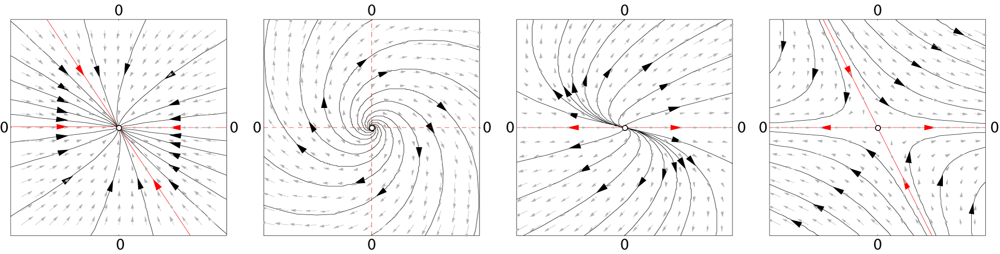
Linear dynamical systems

Main article: Linear dynamical system

Linear dynamical systems can be solved in terms of simple functions and the behavior of all orbits classified. In a linear system the phase space is the N-dimensional Euclidean space, so any point in phase space can be represented by a vector with N numbers. The analysis of linear systems is possible because they satisfy a superposition principle: if u(t) and w(t) satisfy the differential equation for the vector field (but not necessarily the initial condition), then so will u(t) + w(t).

Flows

For a flow, the vector field Φ(x) is a linear function of the position in the phase space, that is,

$\phi(x) = A x + b,\,$

with A a matrix, b a vector of numbers and x the position vector. The solution to this system can be found by using the superposition principle (linearity). The case b ≠ 0 with A = 0 is just a straight line in the direction of b:

$\Phi^t(x_1) = x_1 + b t. \,$

When b is zero and A ≠ 0 the origin is an equilibrium (or singular) point of the flow, that is, if x₀ = 0, then the orbit remains there. For other initial conditions, the equation of motion is given by the exponential of a matrix: for an initial point x₀,

$\Phi^t(x_0) = e^{t A} x_0. \,$

When b = 0, the eigenvalues of A determine the structure of the phase space. From the eigenvalues and the eigenvectors of A it is possible to determine if an initial point will converge or diverge to the equilibrium point at the origin.

The distance between two different initial conditions in the case A ≠ 0 will change exponentially in most cases, either converging exponentially fast towards a point, or diverging exponentially fast. Linear systems display sensitive dependence on initial conditions in the case of divergence. For nonlinear systems this is one of the (necessary but not sufficient) conditions for chaotic behavior.

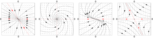Linear vector fields and a few trajectories.

Maps

A discrete-time, affine dynamical system has the form

$x_{n+1} = A x_n + b, \,$

with A a matrix and b a vector. As in the continuous case, the change of coordinates x → x + (1 − A) ^–1b removes the term b from the equation. In the new coordinate system, the origin is a fixed point of the map and the solutions are of the linear system A ⁿx₀. The solutions for the map are no longer curves, but points that hop in the phase space. The orbits are organized in curves, or fibers, which are collections of points that map into themselves under the action of the map.

As in the continuous case, the eigenvalues and eigenvectors of A determine the structure of phase space. For example, if u₁ is an eigenvector of A, with a real eigenvalue smaller than one, then the straight lines given by the points along α u₁, with α ∈ R, is an invariant curve of the map. Points in this straight line run into the fixed point.

There are also many other discrete dynamical systems.

Local dynamics

The qualitative properties of dynamical systems do not change under a smooth change of coordinates (this is sometimes taken as a definition of qualitative): a singular point of the vector field (a point where v(x) = 0) will remain a singular point under smooth transformations; a periodic orbit is a loop in phase space and smooth deformations of the phase space cannot alter it being a loop. It is in the neighborhood of singular points and periodic orbits that the structure of a phase space of a dynamical system can be well understood. In the qualitative study of dynamical systems, the approach is to show that there is a change of coordinates (usually unspecified, but computable) that makes the dynamical system as simple as possible.

Rectification

A flow in most small patches of the phase space can be made very simple. If y is a point where the vector field v(y) ≠ 0, then there is a change of coordinates for a region around y where the vector field becomes a series of parallel vectors of the same magnitude. This is known as the rectification theorem.

The rectification theorem says that away from singular points the dynamics of a point in a small patch is a straight line. The patch can sometimes be enlarged by stitching several patches together, and when this works out in the whole phase space M the dynamical system is integrable. In most cases the patch cannot be extended to the entire phase space. There may be singular points in the vector field (where v(x) = 0); or the patches may become smaller and smaller as some point is approached. The more subtle reason is a global constraint, where the trajectory starts out in a patch, and after visiting a series of other patches comes back to the original one. If the next time the orbit loops around phase space in a different way, then it is impossible to rectify the vector field in the whole series of patches.

Near periodic orbits

In general, in the neighborhood of a periodic orbit the rectification theorem cannot be used. Poincaré developed an approach that transforms the analysis near a periodic orbit to the analysis of a map. Pick a point x₀ in the orbit γ and consider the points in phase space in that neighborhood that are perpendicular to v(x₀). These points are a Poincaré section S(γ, x₀), of the orbit. The flow now defines a map, the Poincaré map F : S → S, for points starting in S and returning to S. Not all these points will take the same amount of time to come back, but the times will be close to the time it takes x₀.

The intersection of the periodic orbit with the Poincaré section is a fixed point of the Poincaré map F. By a translation, the point can be assumed to be at x = 0. The Taylor series of the map is F(x) = J · x + O(x²), so a change of coordinates h can only be expected to simplify F to its linear part

$h^{-1} \circ F \circ h(x) = J \cdot x.\,$

This is known as the conjugation equation. Finding conditions for this equation to hold has been one of the major tasks of research in dynamical systems. Poincaré first approached it assuming all functions to be analytic and in the process discovered the non-resonant condition. If λ₁, ..., λ_ν are the eigenvalues of J they will be resonant if one eigenvalue is an integer linear combination of two or more of the others. As terms of the form λ_i – ∑ (multiples of other eigenvalues) occurs in the denominator of the terms for the function h, the non-resonant condition is also known as the small divisor problem.

Conjugation results

The results on the existence of a solution to the conjugation equation depend on the eigenvalues of J and the degree of smoothness required from h. As J does not need to have any special symmetries, its eigenvalues will typically be complex numbers. When the eigenvalues of J are not in the unit circle, the dynamics near the fixed point x₀ of F is called hyperbolic and when the eigenvalues are on the unit circle and complex, the dynamics is called elliptic.

In the hyperbolic case the Hartman–Grobman theorem gives the conditions for the existence of a continuous function that maps the neighborhood of the fixed point of the map to the linear map J · x. The hyperbolic case is also structurally stable. Small changes in the vector field will only produce small changes in the Poincaré map and these small changes will reflect in small changes in the position of the eigenvalues of J in the complex plane, implying that the map is still hyperbolic.

The Kolmogorov–Arnold–Moser (KAM) theorem gives the behavior near an elliptic point.

Bifurcation theory

Main article: Bifurcation theory

When the evolution map Φ^t (or the vector field it is derived from) depends on a parameter μ, the structure of the phase space will also depend on this parameter. Small changes may produce no qualitative changes in the phase space until a special value μ₀ is reached. At this point the phase space changes qualitatively and the dynamical system is said to have gone through a bifurcation.

Bifurcation theory considers a structure in phase space (typically a fixed point, a periodic orbit, or an invariant torus) and studies its behavior as a function of the parameter μ. At the bifurcation point the structure may change its stability, split into new structures, or merge with other structures. By using Taylor series approximations of the maps and an understanding of the differences that may be eliminated by a change of coordinates, it is possible to catalog the bifurcations of dynamical systems.

The bifurcations of a hyperbolic fixed point x₀ of a system family F_μ can be characterized by the eigenvalues of the first derivative of the system DF_μ(x₀) computed at the bifurcation point. For a map, the bifurcation will occur when there are eigenvalues of DF_μ on the unit circle. For a flow, it will occur when there are eigenvalues on the imaginary axis. For more information, see the main article on Bifurcation theory.

Some bifurcations can lead to very complicated structures in phase space. For example, the Ruelle–Takens scenario describes how a periodic orbit bifurcates into a torus and the torus into a strange attractor. In another example, Feigenbaum period-doubling describes how a stable periodic orbit goes through a series of period-doubling bifurcations.

Ergodic systems

Main article: Ergodic theory

In many dynamical systems it is possible to choose the coordinates of the system so that the volume (really a ν-dimensional volume) in phase space is invariant. This happens for mechanical systems derived from Newton's laws as long as the coordinates are the position and the momentum and the volume is measured in units of (position) × (momentum). The flow takes points of a subset A into the points Φ ^t(A) and invariance of the phase space means that

$\mathrm{vol} (A) = \mathrm{vol} ( \Phi^t(A) ). \,$

In the Hamiltonian formalism, given a coordinate it is possible to derive the appropriate (generalized) momentum such that the associated volume is preserved by the flow. The volume is said to be computed by the Liouville measure.

In a Hamiltonian system not all possible configurations of position and momentum can be reached from an initial condition. Because of energy conservation, only the states with the same energy as the initial condition are accessible. The states with the same energy form an energy shell Ω, a sub-manifold of the phase space. The volume of the energy shell, computed using the Liouville measure, is preserved under evolution.

For systems where the volume is preserved by the flow, Poincaré discovered the recurrence theorem: Assume the phase space has a finite Liouville volume and let F be a phase space volume-preserving map and A a subset of the phase space. Then almost every point of A returns to A infinitely often. The Poincaré recurrence theorem was used by Zermelo to object to Boltzmann's derivation of the increase in entropy in a dynamical system of colliding atoms.

One of the questions raised by Boltzmann's work was the possible equality between time averages and space averages, what he called the ergodic hypothesis. The hypothesis states that the length of time a typical trajectory spends in a region A is vol(A)/vol(Ω).

The ergodic hypothesis turned out not to be the essential property needed for the development of statistical mechanics and a series of other ergodic-like properties were introduced to capture the relevant aspects of physical systems. Koopman approached the study of ergodic systems by the use of functional analysis. An observable a is a function that to each point of the phase space associates a number (say instantaneous pressure, or average height). The value of an observable can be computed at another time by using the evolution function φ ^t. This introduces an operator U ^t, the transfer operator,

$(U^t a)(x) = a(\Phi^{-t}(x)). \,$

By studying the spectral properties of the linear operator U it becomes possible to classify the ergodic properties of Φ ^t. In using the Koopman approach of considering the action of the flow on an observable function, the finite-dimensional nonlinear problem involving Φ ^t gets mapped into an infinite-dimensional linear problem involving U.

The Liouville measure restricted to the energy surface Ω is the basis for the averages computed in equilibrium statistical mechanics. An average in time along a trajectory is equivalent to an average in space computed with the Boltzmann factor exp(−βH). This idea has been generalized by Sinai, Bowen, and Ruelle (SRB) to a larger class of dynamical systems that includes dissipative systems. SRB measures replace the Boltzmann factor and they are defined on attractors of chaotic systems.

Nonlinear dynamical systems and chaos

Main article: Chaos theory

Simple nonlinear dynamical systems and even piecewise linear systems can exhibit a completely unpredictable behavior, which might seem to be random, despite the fact that they are fundamentally deterministic. This seemingly unpredictable behavior has been called chaos. Hyperbolic systems are precisely defined dynamical systems that exhibit the properties ascribed to chaotic systems. In hyperbolic systems the tangent space perpendicular to a trajectory can be well separated into two parts: one with the points that converge towards the orbit (the stable manifold) and another of the points that diverge from the orbit (the unstable manifold).

This branch of mathematics deals with the long-term qualitative behavior of dynamical systems. Here, the focus is not on finding precise solutions to the equations defining the dynamical system (which is often hopeless), but rather to answer questions like "Will the system settle down to a steady state in the long term, and if so, what are the possible attractors?" or "Does the long-term behavior of the system depend on its initial condition?"

Note that the chaotic behavior of complex systems is not the issue. Meteorology has been known for years to involve complex—even chaotic—behavior. Chaos theory has been so surprising because chaos can be found within almost trivial systems. The logistic map is only a second-degree polynomial; the horseshoe map is piecewise linear.

Geometrical definition

A dynamical system is the tuple $\langle \mathcal{M}, f , \mathcal{T}\rangle$, with $\mathcal{M}$ a manifold (locally a Banach space or Euclidean space), $\mathcal{T}$ the domain for time (non-negative reals, the integers, ...) and f an evolution rule t → f ^t (with $t\in\mathcal{T}$) such that f ^t is a diffeomorphism of the manifold to itself. So, f is a mapping of the time-domain $\mathcal{T}$ into the space of diffeomorphisms of the manifold to itself. In other terms, f(t) is a diffeomorphism, for every time t in the domain $\mathcal{T}$ .

Measure theoretical definition

See main article Measure-preserving dynamical system.

A dynamical system may be defined formally, as a measure-preserving transformation of a sigma-algebra, the quadruplet (X,Σ,μ,τ). Here, X is a set, and Σ is a sigma-algebra on X, so that the pair (X,Σ) is a measurable space. μ is a finite measure on the sigma-algebra, so that the triplet (X,Σ,μ) is a probability space. A map $\tau:X\to X$ is said to be Σ-measurable if and only if, for every $\sigma \in \Sigma$, one has $\tau^{-1}\sigma \in \Sigma$. A map τ is said to preserve the measure if and only if, for every $\sigma \in \Sigma$, one has μ(τ ^{− 1}σ) = μ(σ). Combining the above, a map τ is said to be a measure-preserving transformation of X , if it is a map from X to itself, it is Σ-measurable, and is measure-preserving. The quadruple (X,Σ,μ,τ), for such a τ, is then defined to be a dynamical system.

The map τ embodies the time evolution of the dynamical system. Thus, for discrete dynamical systems the iterates $\tau^n=\tau \circ \tau \circ \ldots\circ\tau$ for integer n are studied. For continuous dynamical systems, the map τ is understood to be a finite time evolution map and the construction is more complicated.

Examples of dynamical systems

Internal links

• Arnold's cat map
• Baker's map is an example of a chaotic piecewise linear map
• Circle map
• Double pendulum
• Billiards and Outer Billiards
• Hénon map
• Horseshoe map
• Irrational rotation
• List of chaotic maps
• Logistic map
• Lorenz system
• Rossler map

External links

• Interactive applet for the Standard and Henon Maps by A. Luhn

Multidimensional generalization

Dynamical systems are defined over a single independent variable, usually thought of as time. A more general class of systems are defined over multiple independent variables and are therefore called multidimensional systems. Such systems are useful for modeling, for example, image processing.

See also

Systems science portal

• Behavioral modeling
• Dynamical systems theory
• Feedback passivation
• List of dynamical system topics
• Oscillation
• People in systems and control
• Sarkovskii's theorem
• System dynamics
• Systems theory

References

Further reading

Works providing a broad coverage:

• Ralph Abraham and Jerrold E. Marsden (1978). Foundations of mechanics. Benjamin–Cummings. ISBN 0-8053-0102-X.  (available as a reprint: ISBN 0-201-40840-6)
• Encyclopaedia of Mathematical Sciences (ISSN 0938-0396) has a sub-series on dynamical systems with reviews of current research.
• Anatole Katok and Boris Hasselblatt (1996). Introduction to the modern theory of dynamical systems. Cambridge. ISBN 0-521-57557-5. 
• Christian Bonatti, Lorenzo J. Díaz, Marcelo Viana (2005). Dynamics Beyond Uniform Hyperbolicity: A Global Geometric and Probabilistic Perspective. Springer. ISBN 3-540-22066-6. 
• Stephen Smale (1967). "Differential dynamical systems". Bulletin of the American Mathematical Society 73: 747–817. doi:10.1090/S0002-9904-1967-11798-1. 

Introductory texts with a unique perspective:

• V. I. Arnold (1982). Mathematical methods of classical mechanics. Springer-Verlag. ISBN 0-387-96890-3. 
• Jacob Palis and Wellington de Melo (1982). Geometric theory of dynamical systems: an introduction. Springer-Verlag. ISBN 0-387-90668-1. 
• David Ruelle (1989). Elements of Differentiable Dynamics and Bifurcation Theory. Academic Press. ISBN 0-12-601710-7. 
• Tim Bedford, Michael Keane and Caroline Series, eds. (1991). Ergodic theory, symbolic dynamics and hyperbolic spaces. Oxford University Press. ISBN 0-19-853390-X. 
• Ralph H. Abraham and Christopher D. Shaw (1992). Dynamics—the geometry of behavior, 2nd edition. Addison-Wesley. ISBN 0-201-56716-4. 

Textbooks

• James Meiss (2007). Differential Dynamical Systems. SIAM. ISBN 0898716357. 
• Steven H. Strogatz (1994). Nonlinear dynamics and chaos: with applications to physics, biology chemistry and engineering. Addison Wesley. ISBN 0-201-54344-3. 
• Kathleen T. Alligood, Tim D. Sauer and James A. Yorke (2000). Chaos. An introduction to dynamical systems. Springer Verlag. ISBN 0-387-94677-2. 
• Morris W. Hirsch, Stephen Smale and Robert Devaney (2003). Differential Equations, dynamical systems, and an introduction to chaos. Academic Press. ISBN 0-12-349703-5. 
• Julien Clinton Sprott (2003). Chaos and time-series analysis. Oxford University Press. ISBN 0-19-850839-5. 
• Oded Galor (2011). Discrete Dynamical Systems. Springer. ISBN 978-3-642-07185-0. 

Popularizations:

• Florin Diacu and Philip Holmes (1996). Celestial Encounters. Princeton. ISBN 0-691-02743-9. 
• James Gleick (1988). Chaos: Making a New Science. Penguin. ISBN 0-14-009250-1. 
• Ivar Ekeland (1990). Mathematics and the Unexpected (Paperback). University Of Chicago Press. ISBN 0-226-19990-8. 
• Ian Stewart (1997). Does God Play Dice? The New Mathematics of Chaos. Penguin. ISBN 0140256024. 

External links

• A collection of dynamic and non-linear system models and demo applets (in Monash University's Virtual Lab)
• Arxiv preprint server has daily submissions of (non-refereed) manuscripts in dynamical systems.
• DSWeb provides up-to-date information on dynamical systems and its applications.
• Encyclopedia of dynamical systems A part of Scholarpedia — peer reviewed and written by invited experts.
• Nonlinear Dynamics. Models of bifurcation and chaos by Elmer G. Wiens
• Oliver Knill has a series of examples of dynamical systems with explanations and interactive controls.
• Sci.Nonlinear FAQ 2.0 (Sept 2003) provides definitions, explanations and resources related to nonlinear science

Online books or lecture notes:

• Geometrical theory of dynamical systems. Nils Berglund's lecture notes for a course at ETH at the advanced undergraduate level.
• Dynamical systems. George D. Birkhoff's 1927 book already takes a modern approach to dynamical systems.
• Chaos: classical and quantum. An introduction to dynamical systems from the periodic orbit point of view.
• Modeling Dynamic Systems. An introduction to the development of mathematical models of dynamic systems.
• Learning Dynamical Systems. Tutorial on learning dynamical systems.
• Ordinary Differential Equations and Dynamical Systems. Lecture notes by Gerald Teschl

Research groups:

• Dynamical Systems Group Groningen, IWI, University of Groningen.
• Chaos @ UMD. Concentrates on the applications of dynamical systems.
• Dynamical Systems, SUNY Stony Brook. Lists of conferences, researchers, and some open problems.
• Center for Dynamics and Geometry, Penn State.
• Control and Dynamical Systems, Caltech.
• Laboratory of Nonlinear Systems, Ecole Polytechnique Fédérale de Lausanne (EPFL).
• Center for Dynamical Systems, University of Bremen
• Systems Analysis, Modelling and Prediction Group, University of Oxford
• Non-Linear Dynamics Group, Instituto Superior Técnico, Technical University of Lisbon
• Dynamical Systems, IMPA, Instituto Nacional de Matemática Pura e Applicada.
• Nonlinear Dynamics Workgroup, Institute of Computer Science, Czech Academy of Sciences.

Simulation software based on Dynamical Systems approach:

• FyDiK
• iDMC, simulation and dynamical analysis of nonlinear models