Computer simulation

This article is about computer model within a scientific context. For artistic usage, see 3d modeling. For simulating a computer on a computer, see emulator.

A 48 hour computer simulation of Typhoon Mawar using the Weather Research and Forecasting model

A computer simulation, a computer model, or a computational model is a computer program, or network of computers, that attempts to simulate an abstract model of a particular system. Computer simulations have become a useful part of mathematical modeling of many natural systems in physics (computational physics), astrophysics, chemistry and biology, human systems in economics, psychology, social science, and engineering. Simulations can be used to explore and gain new insights into new technology, and to estimate the performance of systems too complex for analytical solutions.^[1]

Computer simulations vary from computer programs that run a few minutes, to network-based groups of computers running for hours, to ongoing simulations that run for days. The scale of events being simulated by computer simulations has far exceeded anything possible (or perhaps even imaginable) using the traditional paper-and-pencil mathematical modeling. Over 10 years ago, a desert-battle simulation, of one force invading another, involved the modeling of 66,239 tanks, trucks and other vehicles on simulated terrain around Kuwait, using multiple supercomputers in the DoD High Performance Computer Modernization Program;^[2] a 1-billion-atom model of material deformation (2002); a 2.64-million-atom model of the complex maker of protein in all organisms, a ribosome, in 2005;^[3] and the Blue Brain project at EPFL (Switzerland), began in May 2005, to create the first computer simulation of the entire human brain, right down to the molecular level.^[4]

Simulation versus modeling

Traditionally, building large models of systems has been via a statistical model, which attempts to find analytical solutions to problems and thereby enable the prediction of the behavior of the system from a set of parameters and initial conditions.

The term computer simulation is broader than computer modeling; the latter implies that all aspects are being modeled in the computer representation. However, computer simulation also includes generating inputs from simulated users in order to run actual computer software or equipment, with only part of the system being modeled. An example would be a flight simulator that can run machines as well as actual flight software.

Computer simulations are used in many fields, including science, technology, entertainment, health care, and business planning and scheduling.

History

Computer simulation developed hand-in-hand with the rapid growth of the computer, following its first large-scale deployment during the Manhattan Project in World War II to model the process of nuclear detonation. It was a simulation of 12 hard spheres using a Monte Carlo algorithm. Computer simulation is often used as an adjunct to, or substitute for, modeling systems for which simple closed form analytic solutions are not possible. There are many types of computer simulations; the common feature they all share is the attempt to generate a sample of representative scenarios for a model in which a complete enumeration of all possible states of the model would be prohibitive or impossible.

Data preparation

The external data requirements of simulations and models vary widely. For some, the input might be just a few numbers (for example, simulation of a waveform of AC electricity on a wire), while others might require terabytes of information (such as weather and climate models).

Input sources also vary widely:

• Sensors and other physical devices connected to the model;
• Control surfaces used to direct the progress of the simulation in some way;
• Current or Historical data entered by hand;
• Values extracted as by-product from other processes;
• Values output for the purpose by other simulations, models, or processes.

Lastly, the time at which data is available varies:

• "invariant" data is often built into the model code, either because the value is truly invariant (e.g. the value of π) or because the designers consider the value to be invariant for all cases of interest;
• data can entered into the simulation when it starts up, for example by reading one or more files, or by reading data from a preprocessor;
• data can be provided during the simulation run, for example by a sensor network;

Because of this variety, and that many common elements exist between diverse simulation systems, there are a large number of specialized simulation languages. The best-known of these may be Simula (sometimes Simula-67, after the year 1967 when it was proposed). There are now many others.

Systems that accept data from external sources must be very careful in knowing what they are receiving. While it is easy for computers to read in values from text or binary files, what is much harder is knowing what the accuracy (compared to measurement resolution and precision) of the values is. Often it is expressed as "error bars", a minimum and maximum deviation from the value seen within which the true value (is expected to) lie. Because digital computer mathematics is not perfect, rounding and truncation errors will multiply this error up, and it is therefore useful to perform an "error analysis"^[5] to check that values output by the simulation are still usefully accurate.

Even small errors in the original data can accumulate into substantial error later in the simulation. While all computer analysis is subject to the "GIGO" (garbage in, garbage out) restriction, this is especially true of digital simulation. Indeed, it was the observation of this inherent, cumulative error, for digital systems that is the origin of chaos theory.

Types

Computer models can be classified according to several independent pairs of attributes, including:

• Stochastic or deterministic (and as a special case of deterministic, chaotic) - see External links below for examples of stochastic vs. deterministic simulations
• Steady-state or dynamic
• Continuous or discrete (and as an important special case of discrete, discrete event or DE models)
• Local or distributed.

Another way of categorizing models is to have a look at the underlying data structures. For time stepped simulations, there are two main classes:

• Simulations which store their data in regular grids and require only next neighbor access are called stencil codes. Many CFD applications belong into this category.
• If the underlying graph is not a regular grid, the model may belong to the meshfree methods.

Equations define the relationships between elements of the modeled system and attempt to find a state in which the system is in equilibrium. Such models are often used in simulating physical systems, as a simpler modeling case before dynamic simulation is attempted.

• Dynamic simulations model changes in a system in response to (usually changing) input signals.
• Stochastic models use random number generators to model chance or random events;
• A discrete event simulation (DES) manages events in time. Most computer, logic-test and fault-tree simulations are of this type. In this type of simulation, the simulator maintains a queue of events sorted by the simulated time they should occur. The simulator reads the queue and triggers new events as each event is processed. It is not important to execute the simulation in real time. It's often more important to be able to access the data produced by the simulation, to discover logic defects in the design, or the sequence of events.
• A continuous dynamic simulation performs numerical solution of differential-algebraic equations or differential equations (either partial or ordinary). Periodically, the simulation program solves all the equations, and uses the numbers to change the state and output of the simulation. Applications include flight simulators, construction and management simulation games, chemical process modeling, and simulations of electrical circuits. Originally, these kinds of simulations were actually implemented on analog computers, where the differential equations could be represented directly by various electrical components such as op-amps. By the late 1980s, however, most "analog" simulations were run on conventional digital computers that emulate the behavior of an analog computer.
• A special type of discrete simulation that does not rely on a model with an underlying equation, but can nonetheless be represented formally, is agent-based simulation. In agent-based simulation, the individual entities (such as molecules, cells, trees or consumers) in the model are represented directly (rather than by their density or concentration) and possess an internal state and set of behaviors or rules that determine how the agent's state is updated from one time-step to the next.
• Distributed models run on a network of interconnected computers, possibly through the Internet. Simulations dispersed across multiple host computers like this are often referred to as "distributed simulations". There are several standards for distributed simulation, including Aggregate Level Simulation Protocol (ALSP), Distributed Interactive Simulation (DIS), the High Level Architecture (simulation) (HLA) and the Test and Training Enabling Architecture (TENA).

CGI computer simulation

Formerly, the output data from a computer simulation was sometimes presented in a table, or a matrix, showing how data was affected by numerous changes in the simulation parameters. The use of the matrix format was related to traditional use of the matrix concept in mathematical models; however, psychologists and others noted that humans could quickly perceive trends by looking at graphs or even moving-images or motion-pictures generated from the data, as displayed by computer-generated-imagery (CGI) animation. Although observers couldn't necessarily read out numbers, or spout math formulas, from observing a moving weather chart, they might be able to predict events (and "see that rain was headed their way"), much faster than scanning tables of rain-cloud coordinates. Such intense graphical displays, which transcended the World of numbers and formulae, sometimes also led to output that lacked a coordinate grid or omitted timestamps, as if straying too far from numeric data displays. Today, weather forecasting models tend to balance the view of moving rain/snow clouds against a map that uses numeric coordinates and numeric timestamps of events.

Similarly, CGI computer simulations of CAT scans can simulate how a tumor might shrink or change, during an extended period of medical treatment, presenting the passage of time as a spinning view of the visible human head, as the tumor changes.

Other applications of CGI computer simulations are being developed to graphically display large amounts of data, in motion, as changes occur during a simulation run.

Computer simulation in science

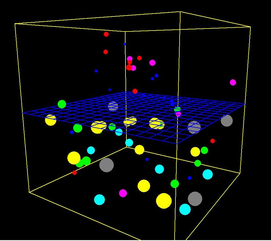
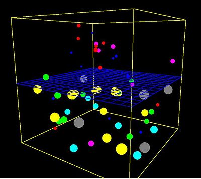Computer simulation of the process of osmosis

Generic examples of types of computer simulations in science, which are derived from an underlying mathematical description:

• a numerical simulation of differential equations that cannot be solved analytically, theories that involve continuous systems such as phenomena in physical cosmology, fluid dynamics (e.g. climate models, roadway noise models, roadway air dispersion models), continuum mechanics and chemical kinetics fall into this category.
• a stochastic simulation, typically used for discrete systems where events occur probabilistically, and which cannot be described directly with differential equations (this is a discrete simulation in the above sense). Phenomena in this category include genetic drift, biochemical or gene regulatory networks with small numbers of molecules. (see also: Monte Carlo method).

Specific examples of computer simulations follow:

• statistical simulations based upon an agglomeration of a large number of input profiles, such as the forecasting of equilibrium temperature of receiving waters, allowing the gamut of meteorological data to be input for a specific locale. This technique was developed for thermal pollution forecasting .
• agent based simulation has been used effectively in ecology, where it is often called individual based modeling and has been used in situations for which individual variability in the agents cannot be neglected, such as population dynamics of salmon and trout (most purely mathematical models assume all trout behave identically).
• time stepped dynamic model. In hydrology there are several such hydrology transport models such as the SWMM and DSSAM Models developed by the U.S. Environmental Protection Agency for river water quality forecasting.
• computer simulations have also been used to formally model theories of human cognition and performance, e.g. ACT-R
• computer simulation using molecular modeling for drug discovery
• computer simulation for studying the selective sensitivity of bonds by mechanochemistry during grinding of organic molecules.^[6]
• Computational fluid dynamics simulations are used to simulate the behaviour of flowing air, water and other fluids. There are one-, two- and three- dimensional models used. A one dimensional model might simulate the effects of water hammer in a pipe. A two-dimensional model might be used to simulate the drag forces on the cross-section of an aeroplane wing. A three-dimensional simulation might estimate the heating and cooling requirements of a large building.
• An understanding of statistical thermodynamic molecular theory is fundamental to the appreciation of molecular solutions. Development of the Potential Distribution Theorem (PDT) allows one to simplify this complex subject to down-to-earth presentations of molecular theory.

Notable, and sometimes controversial, computer simulations used in science include: Donella Meadows' World3 used in the Limits to Growth, James Lovelock's Daisyworld and Thomas Ray's Tierra.

Simulation environments for physics and engineering

Graphical environments to design simulations have been developed. Special care was taken to handle events (situations in which the simulation equations are not valid and have to be changed). The open project Open Source Physics was started to develop reusable libraries for simulations in Java, together with Easy Java Simulations, a complete graphical environment that generates code based on these libraries.

Computer simulation in practical contexts

Smog around Karl Marx Stadt (Chemnitz), Germany: computer simulation in 1990

Computer simulations are used in a wide variety of practical contexts, such as:

• analysis of air pollutant dispersion using atmospheric dispersion modeling
• design of complex systems such as aircraft and also logistics systems.
• design of Noise barriers to effect roadway noise mitigation
• flight simulators to train pilots
• weather forecasting
• Simulation of other computers is emulation.
• forecasting of prices on financial markets (for example Adaptive Modeler)
• behavior of structures (such as buildings and industrial parts) under stress and other conditions
• design of industrial processes, such as chemical processing plants
• Strategic Management and Organizational Studies
• Reservoir simulation for the petroleum engineering to model the subsurface reservoir
• Process Engineering Simulation tools.
• Robot simulators for the design of robots and robot control algorithms
• Urban Simulation Models that simulate dynamic patterns of urban development and responses to urban land use and transportation policies. See a more detailed article on Urban Environment Simulation.
• Traffic engineering to plan or redesign parts of the street network from single junctions over cities to a national highway network, for transportation system planning, design and operations. See a more detailed article on Simulation in Transportation.
• modeling car crashes to test safety mechanisms in new vehicle models

The reliability and the trust people put in computer simulations depends on the validity of the simulation model, therefore verification and validation are of crucial importance in the development of computer simulations. Another important aspect of computer simulations is that of reproducibility of the results, meaning that a simulation model should not provide a different answer for each execution. Although this might seem obvious, this is a special point of attention in stochastic simulations, where random numbers should actually be semi-random numbers. An exception to reproducibility are human in the loop simulations such as flight simulations and computer games. Here a human is part of the simulation and thus influences the outcome in a way that is hard, if not impossible, to reproduce exactly.

Vehicle manufacturers make use of computer simulation to test safety features in new designs. By building a copy of the car in a physics simulation environment, they can save the hundreds of thousands of dollars that would otherwise be required to build a unique prototype and test it. Engineers can step through the simulation milliseconds at a time to determine the exact stresses being put upon each section of the prototype.^[7]

Computer graphics can be used to display the results of a computer simulation. Animations can be used to experience a simulation in real-time e.g. in training simulations. In some cases animations may also be useful in faster than real-time or even slower than real-time modes. For example, faster than real-time animations can be useful in visualizing the buildup of queues in the simulation of humans evacuating a building. Furthermore, simulation results are often aggregated into static images using various ways of scientific visualization.

In debugging, simulating a program execution under test (rather than executing natively) can detect far more errors than the hardware itself can detect and, at the same time, log useful debugging information such as instruction trace, memory alterations and instruction counts. This technique can also detect buffer overflow and similar "hard to detect" errors as well as produce performance information and tuning data.

Pitfalls

Although sometimes ignored in computer simulations, it is very important to perform sensitivity analysis to ensure that the accuracy of the results are properly understood. For example, the probabilistic risk analysis of factors determining the success of an oilfield exploration program involves combining samples from a variety of statistical distributions using the Monte Carlo method. If, for instance, one of the key parameters (e.g. the net ratio of oil-bearing strata) is known to only one significant figure, then the result of the simulation might not be more precise than one significant figure, although it might (misleadingly) be presented as having four significant figures.

Model Calibration Techniques

The following three steps should be used to produce accurate simulation models: calibration, verification, and validation. Computer simulations are good at portraying and comparing theoretical scenarios but in order to accurately model actual case studies, it has to match what is actually happening today. A base model should be created and calibrated so that it matches the area being studied. The calibrated model should then be verified to ensure that the model is operating as expected based on the inputs. Once the model has been verified, the final step is to validate the model by comparing the outputs to historical data from the study area. This can be done by using statistical techniques and ensuring an adequate R-squared value. Unless these techniques are employed, the simulation model created will produce inaccurate results and not be a useful prediction tool.

Model calibration is achieved by adjusting any available parameters in order to adjust how the model operates and simulates the process. For example in traffic simulation, typical parameters include look-ahead distance, car-following sensitivity, discharge headway, and start-up lost time. These parameters influence driver behaviors such as when and how long it takes a driver to change lanes, how much distance a driver leaves between itself and the car in front of it, and how quickly it starts to accelerate through an intersection. Adjusting these parameters has a direct effect on the amount of traffic volume that can traverse through the modeled roadway network by making the drivers more or less aggressive. These are examples of calibration parameters that can be fine-tuned to match up with characteristics observed in the field at the study location. Most traffic models will have typical default values but they may need to be adjusted to better match the driver behavior at the location being studied.

Model verification is achieved by obtaining output data from the model and comparing it to what is expected from the input data. For example in traffic simulation, traffic volume can be verified to ensure that actual volume throughput in the model is reasonably close to traffic volumes input into the model. Ten percent is a typical threshold used in traffic simulation to determine if output volumes are reasonably close to input volumes. Simulation models handle model inputs in different ways so traffic that enters the network, for example, may or may not reach its desired destination. Additionally, traffic that wants to enter the network may not be able to, if any congestion exists. This is why model verification is a very important part of the modeling process.

The final step is to validate the model by comparing the results with what’s expected based on historical data from the study area. Ideally, the model should produce similar results to what has happened historically. This is typically verified by nothing more than quoting the R2 statistic from the fit. This statistic measures the fraction of variability that is accounted for by the model. A high R2 value does not necessarily mean the model fits the data well. Another tool used to validate models is graphical residual analysis. If model output values are drastically different than historical values, it probably means there’s an error in the model. This is an important step to verify before using the model as a base to produce additional models for different scenarios to ensure each one is accurate. If the outputs do not reasonably match historic values during the validation process, the model should be reviewed and updated to produce results more in line with expectations. It is an iterative process that helps to produce more realistic models.

Validating traffic simulation models requires comparing traffic estimated by the model to observed traffic on the roadway and transit systems. Initial comparisons are for trip interchanges between quadrants, sectors, or other large areas of interest. The next step is to compare traffic estimated by the models to traffic counts, including transit ridership, crossing contrived barriers in the study area. These are typically called screenlines, cutlines, and cordon lines and may be imaginary or actual physical barriers. Cordon lines surround particular areas such as the central business district or other major activity centers. Transit ridership estimates are commonly validated by comparing them to actual patronage crossing cordon lines around the central business district.

Three sources of error can cause weak correlation during calibration: input error, model error, and parameter error. In general, input error and parameter error can be adjusted easily by the user. Model error however is caused by the methodology used in the model and may not be as easy to fix. Simulation models are typically built using several different modeling theories that can produce conflicting results. Some models are more generalized while others are more detailed. If model error occurs as a result of this, in may be necessary to adjust the model methodology to make results more consistent.

In order to produce good models that can be used to produce realistic results, these are the necessary steps that need to be taken in order to ensure that simulation models are functioning properly. Simulation models can be used as a tool to verify engineering theories but are only valid, if calibrated properly. Once satisfactory estimates of the parameters for all models have been obtained, the models must be checked to assure that they adequately perform the functions for which they are intended. The validation process establishes the credibility of the model by demonstrating its ability to replicate actual traffic patterns. The importance of model validation underscores the need for careful planning, thoroughness and accuracy of the input data collection program that has this purpose. Efforts should be made to ensure collected data is consistent with expected values. For example in traffic analysis, it is typically common for a traffic engineer to perform a site visit to verify traffic counts and become familiar with traffic patterns in the area. The resulting models and forecasts will be no better than the data used for model estimation and validation.

See also

• Virtual prototyping
• Stencil codes
• Meshfree methods
• Web-based simulation
• Emulator
• Procedural animation

References

1. ^ Strogatz, Steven (2007). "The End of Insight". In Brockman, John. What is your dangerous idea?. HarperCollins. ISSN 9780061214950 
2. ^ " "Researchers stage largest Military Simulation ever", Jet Propulsion Laboratory, Caltech, December 1997,
3. ^ "Largest computational biology simulation mimics life's most essential nanomachine" (news), News Release, Nancy Ambrosiano, Los Alamos National Laboratory, Los Alamos, NM, October 2005, webpage: LANL-Fuse-story7428.
4. ^ "Mission to build a simulated brain begins", project of the institute at the École Polytechnique Fédérale de Lausanne (EPFL), Switzerland, New Scientist, June 2005.
5. ^ John Robert Taylor (1999). An Introduction to Error Analysis: The Study of Uncertainties in Physical Measurements. University Science Books. pp. 128–129. ISBN 093570275X. http://books.google.com/books?id=giFQcZub80oC&pg=PA128. 
6. ^ Mizukami, Koichi ; Saito, Fumio ; Baron, Michel. Study on grinding of pharmaceutical products with an aid of computer simulation
7. ^ Baase, Sara. A Gift of Fire: Social, Legal, and Ethical Issues for Computing and the Internet. 3. Upper Saddle River: Prentice Hall, 2007. Pages 363-364. ISBN 0-13-600848-8.

Notes

• R. Frigg and S. Hartmann, Models in Science. Entry in the Stanford Encyclopedia of Philosophy.
• S. Hartmann, The World as a Process: Simulations in the Natural and Social Sciences, in: R. Hegselmann et al. (eds.), Modelling and Simulation in the Social Sciences from the Philosophy of Science Point of View, Theory and Decision Library. Dordrecht: Kluwer 1996, 77-100.
• P. Humphreys, Extending Ourselves: Computational Science, Empiricism, and Scientific Method. Oxford: Oxford University Press, 2004.
• James J. Nutaro, Building Software for Simulation: Theory and Algorithms, with Applications in C++. Wiley, 2010.