Hardy–Weinberg principle

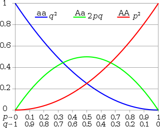Hardy–Weinberg principle for two alleles: the horizontal axis shows the two allele frequencies p and q and the vertical axis shows the genotype frequencies. Each graph shows one of the three possible genotypes.

The Hardy–Weinberg principle (also known by a variety of names: HWP, Hardy–Weinberg equilibrium, Hardy–Weinberg Theorem, HWE, or Hardy–Weinberg law) states that both allele and genotype frequencies in a population remain constant—that is, they are in equilibrium—from generation to generation unless specific disturbing influences are introduced. Those disturbing influences include non-random mating, mutations, selection, limited population size, "overlapping generations", random genetic drift, gene flow and meiotic drive. It is important to understand that outside the lab, one or more of these "disturbing influences" are always in effect. That is, Hardy–Weinberg equilibrium is impossible in nature. Genetic equilibrium is an ideal state that provides a baseline against which to measure change.

Static allele frequencies in a population across generations assume: no mutation (the alleles don't change), no migration or emigration (no exchange of alleles between populations), infinitely large population size, and no selective pressure for or against any genotypes. Genotype frequencies will also be static when mating is random.

In the simplest case of a single locus with two alleles: the dominant allele is denoted A and the recessive a and their frequencies are denoted by p and q; freq(A) = p; freq(a) = q; p + q = 1. If the population is in equilibrium, then we will have freq(AA) = p² for the AA homozygotes in the population, freq(aa) = q² for the aa homozygotes, and freq(Aa) = 2pq for the heterozygotes.

This concept was named after G. H. Hardy and Wilhelm Weinberg.

Derivation

A better, but equivalent, probabilistic description for the HWP is that the alleles for the next generation for any given individual are chosen randomly and independent of each other. Consider two alleles, A and a, with frequencies p and q, respectively, in the population. The different ways to form new genotypes can be derived using a Punnett square, where the fraction in each is equal to the product of the row and column probabilities.

Table 1: Punnett square for Hardy–Weinberg equilibrium

		Females
		A (p)	a (q)
Males	A (p)	AA (p2)	Aa (pq)
	a (q)	Aa (pq)	aa (q2)

The formula is sometimes written as (p²) + (2pq) + (q²) = 1, representing the fact that probabilities (normalised frequencies for a theoretically infinite population size) must add up to one.

The final three possible genotypic frequencies in the offspring become:

• $f(\mathbf{AA}) = p^2\,$
• $f(\mathbf{Aa}) = 2pq\,$
• $f(\mathbf{aa}) = q^2\,$

These frequencies are called Hardy–Weinberg frequencies (or Hardy–Weinberg proportions). This is achieved in one generation, and only requires the assumption of random mating with an infinite population size.

Sometimes, a population is created by bringing together males and females with different allele frequencies. In this case, the assumption of a single population is violated until after the first generation, so the first generation will not have Hardy–Weinberg equilibrium. Successive generations will have Hardy–Weinberg equilibrium.

Deviations from Hardy–Weinberg equilibrium

Violations of the Hardy–Weinberg assumptions can cause deviations from expectation. How this affects the population depends on the assumptions that are violated. Generally, deviation from the Hardy–Weinberg equilibrium denotes the evolution of a species.

• Random mating. The HWP states the population will have the given genotypic frequencies (called Hardy–Weinberg proportions) after a single generation of random mating within the population. When violations of this provision occur, the population will not have Hardy–Weinberg proportions. Three such violations are:
  • Inbreeding, which causes an increase in homozygosity for all genes.
  • Assortative mating, which causes an increase in homozygosity only for those genes involved in the trait that is assortatively mated (and genes in linkage disequilibrium with them).
  • Small population size, which causes a random change in genotypic frequencies. This is due to a sampling effect, and is called genetic drift. Sampling effects are most important when population sizes are small or the allele is rare.

If a population violates one of the following four assumptions, the population may continue to have Hardy–Weinberg proportions each generation, but the allele frequencies will change with that force.

• Selection, in general, causes allele frequencies to change, often quite rapidly. While directional selection eventually leads to the loss of all alleles except the favored one, some forms of selection, such as balancing selection, lead to equilibrium without loss of alleles.
• Mutation will have a very subtle effect on allele frequencies. Mutation rates are of the order 10⁻⁴ to 10⁻⁸, and the change in allele frequency will be, at most, the same order. Recurrent mutation will maintain alleles in the population, even if there is strong selection against them.
• Migration genetically links two or more populations together. In general, allele frequencies will become more homogeneous among the populations. Some models for migration inherently include nonrandom mating (Wahlund effect, for example). For those models, the Hardy–Weinberg proportions will normally not be valid.

How these violations affect formal statistical tests for HWE is discussed later.

Unfortunately, violations of assumptions in the Hardy–Weinberg principle does not mean the population will violate HWE. For example, balancing selection leads to an equilibrium population with Hardy–Weinberg proportions. This property with selection vs. mutation is the basis for many estimates of mutation rate (call mutation-selection balance).

Sex linkage

Where the A gene is sex linked, the heterogametic sex (e.g., mammalian males; avian females) have only one copy of the gene (and are termed hemizygous), while the homogametic sex (e.g., human females) have two copies. The genotype frequencies at equilibrium are p and q for the heterogametic sex but p², 2pq and q² for the homogametic sex.

For example, in humans red–green colorblindness is an X-linked recessive trait. In western European males, the trait affects about 1 in 12, (q = 0.083) whereas it affects about 1 in 200 females (0.005, compared to q² = 0.007), very close to Hardy–Weinberg proportions.

If a population is brought together with males and females with different allele frequencies, the allele frequency of the male population follows that of the female population because each receives its X chromosome from its mother. The population converges on equilibrium very quickly.

Generalizations

The simple derivation above can be generalized for more than two alleles and polyploidy.

Generalization for more than two alleles

Consider an extra allele frequency, r. The two-allele case is the binomial expansion of (p + q)², and thus the three-allele case is the trinomial expansion of (p + q+ r)².

$(p+q+r)^2=p^2 + r^2 + q^2 + 2pq +2pr + 2qr\,$

More generally, consider the alleles A₁, ..., A_i given by the allele frequencies p₁ to p_i;

$(p_1 + \cdots + p_i)^2\,$

giving for all homozygotes:

$f(A_i A_i) = p_i^2\,$

and for all heterozygotes:

$f(A_i A_j) = 2p_ip_j\,$

Generalization for polyploidy

The Hardy–Weinberg principle may also be generalized to polyploid systems, that is, for organisms that have more than two copies of each chromosome. Consider again only two alleles. The diploid case is the binomial expansion of:

$(p + q)^2\,$

and therefore the polyploid case is the polynomial expansion of:

$(p + q)^c\,$

where c is the ploidy, for example with tetraploid (c = 4):

Table 2: Expected genotype frequencies for tetraploidy

Genotype	Frequency
$\mathbf A \mathbf A \mathbf A \mathbf A$	p4
$\mathbf A \mathbf A \mathbf A \mathbf a$	4p3q
$\mathbf A \mathbf A \mathbf a \mathbf a$	6p2q2
$\mathbf A \mathbf a \mathbf a \mathbf a$	4pq3
$\mathbf a \mathbf a \mathbf a \mathbf a$	q4

Depending on whether the organism is a 'true' tetraploid or an amphidiploid will determine how long it will take for the population to reach Hardy–Weinberg equilibrium.

Complete generalization

For n distinct alleles in c-ploids, the genotype frequencies in the Hardy–Weinberg equilibrium are given by individual terms in the multinomial expansion of $(p_1 + \cdots + p_n)^c$:

$(p_1 + \cdots + p_n)^c = \sum_{k_1, \ldots, k_n\ \in \mathbb{N} : k_1 + \cdots +k_n=c} {c \choose k_1, \ldots, k_n} p_1^{k_1} \cdots p_n^{k_n}$

Applications

The Hardy–Weinberg principle may be applied in two ways, either a population is assumed to be in Hardy–Weinberg proportions, in which the genotype frequencies can be calculated, or if the genotype frequencies of all three genotypes are known, they can be tested for deviations that are statistically significant.

Application to cases of complete dominance

Suppose that the phenotypes of AA and Aa are indistinguishable, i.e., there is complete dominance. Assuming that the Hardy–Weinberg principle applies to the population, then q can still be calculated from f(aa):

$q = \sqrt {f(aa)}$

and p can be calculated from q. And thus an estimate of f(AA) and f(Aa) derived from p² and 2pq respectively. Note however, such a population cannot be tested for equilibrium using the significance tests below because it is assumed a priori.

Significance tests for deviation

Testing deviation from the HWP is generally performed using Pearson's chi-squared test, using the observed genotype frequencies obtained from the data and the expected genotype frequencies obtained using the HWP. For systems where there are large numbers of alleles, this may result in data with many empty possible genotypes and low genotype counts, because there are often not enough individuals present in the sample to adequately represent all genotype classes. If this is the case, then the asymptotic assumption of the chi-squared distribution, will no longer hold, and it may be necessary to use a form of Fisher's exact test, which requires a computer to solve. More recently a number of MCMC methods of testing for deviations from HWP have been proposed (Guo & Thompson, 1992; Wigginton et al. 2005)

Example χ² test for deviation

These data are from E.B. Ford (1971) on the Scarlet tiger moth, for which the phenotypes of a sample of the population were recorded. Genotype-phenotype distinction is assumed to be negligibly small. The null hypothesis is that the population is in Hardy–Weinberg proportions, and the alternative hypothesis is that the population is not in Hardy–Weinberg proportions.

Table 3: Example Hardy–Weinberg principle calculation

Phenotype	White-spotted (AA)	Intermediate (Aa)	Little spotting (aa)	Total
Number	1469	138	5	1612

From which allele frequencies can be calculated:

$\begin{align} p & = {2 \times \mathrm{obs}(AA) + \mathrm{obs}(Aa) \over 2 \times (\mathrm{obs}(AA) + \mathrm{obs}(Aa) + \mathrm{obs}(aa))} \\ \\ & = {1469 \times 2 + 138 \over 2 \times (1469+138+5)} \\ \\ & = { 3076 \over 3224} \\ \\ & = 0.954 \end{align}$

and

$\begin{align} q & = 1 - p \\ & = 1 - 0.954 \\ & = 0.046 \end{align}$

So the Hardy–Weinberg expectation is:

$\begin{align} \mathrm{Exp}(AA) & = p^2n = 0.954^2 \times 1612 = 1467.4 \\ \mathrm{Exp}(Aa) & = 2pqn = 2 \times 0.954 \times 0.046 \times 1612 = 141.2 \\ \mathrm{Exp}(aa) & = q^2n = 0.046^2 \times 1612 = 3.4 \end{align}$

Pearson's chi-squared test states:

$\begin{align} \chi^2 & = \sum {(O - E)^2 \over E} \\ & = {(1469 - 1467.4)^2 \over 1467.4} + {(138 - 141.2)^2 \over 141.2} + {(5 - 3.4)^2 \over 3.4} \\ & = 0.001 + 0.073 + 0.756 \\ & = 0.83 \end{align}$

There is 1 degree of freedom (degrees of freedom for test for Hardy–Weinberg proportions are # genotypes − # alleles). The 5% significance level for 1 degree of freedom is 3.84, and since the χ² value is less than this, the null hypothesis that the population is in Hardy–Weinberg frequencies is not rejected.

Fisher's exact test (probability test)

Fisher's exact test can be applied to testing for Hardy–Weinberg proportions. Because the test is conditional on the allele frequencies, p and q, the problem can be viewed as testing for the proper number of heterozygotes. In this way, the hypothesis of Hardy–Weinberg proportions is rejected if the number of heterozygotes are too large or too small. The conditional probabilities for the heterozygote, given the allele frequencies are given in Emigh (1980) as

$\operatorname{prob}[n_{12} | n_1] = \frac{{n\choose n_{11}, n_{12}, n_{22} }} {{2n \choose n_1}} 2^{n_{12}},$

where n₁₁, n₁₂, n₂₂ are the observed numbers of the three genotypes, AA, Aa, and aa, respectively, and n₁ is the number of A alleles, where n₁ = 2n₁₁ + n₁₂.

An example Using one of the examples from Emigh (1980),^[1] we can consider the case where n = 100, and p = 0.34. The possible observed heterozygotes and their exact significance level is given in Table 4.

Table 4: Example of Fisher's Exact Test for n = 100, p = 0.34.^[1]

Number of heterozygotes	Significance level
0	0.000
2	0.000
4	0.000
6	0.000
8	0.000
10	0.000
12	0.000
14	0.000
16	0.000
18	0.001
20	0.007
22	0.034
24	0.067
26	0.151
28	0.291
30	0.474
32	0.730
34	1.000

Using this table, you look up the significance level of the test based on the observed number of heterozygotes. For example, if you observed 20 heterozygotes, the significance level for the test is 0.007. As is typical for Fisher's exact test for small samples, the gradation of significance levels is quite coarse.

Unfortunately, you have to create a table like this for every experiment, since the tables are dependent on both n and p.

Inbreeding coefficient

The inbreeding coefficient, F (see also F-statistics), is one minus the observed frequency of heterozygotes over that expected from Hardy–Weinberg equilibrium.

$F = \frac{\operatorname{E}{(f(\mathbf{Aa}))} - \operatorname{O}(f(\mathbf{Aa}))} {\operatorname{E}(f(\mathbf{Aa}))} = 1 - \frac{\operatorname{O}(f(\mathbf{Aa}))} {\operatorname{E}(f(\mathbf{Aa}))} , \!$

where the expected value from Hardy–Weinberg equilibrium is given by

$\operatorname{E}(f(\mathbf{Aa})) = 2\, p\, q\, \!$

For example, for Ford's data above;

$F = 1 - {138 \over 141.2} = 0.023.\,$

For two alleles, the chi-squared goodness of fit test for Hardy–Weinberg proportions is equivalent to the test for inbreeding, F = 0.

The inbreeding coefficient is unstable as the expected value approaches zero, and thus not useful for rare and very common alleles. For: E = 0, O > 0, F = −∞ and E = 0, O = 0, F is undefined.

History

Mendelian genetics were rediscovered in 1900. However, it remained somewhat controversial for several years as it was not then known how it could cause continuous characteristics. Udny Yule (1902) argued against Mendelism because he thought that dominant alleles would increase in the population. The American William E. Castle (1903) showed that without selection, the genotype frequencies would remain stable. Karl Pearson (1903) found one equilibrium position with values of p = q = 0.5. Reginald Punnett, unable to counter Yule's point, introduced the problem to G. H. Hardy, a British mathematician, with whom he played cricket. Hardy was a pure mathematician and held applied mathematics in some contempt; his view of biologists' use of mathematics comes across in his 1908 paper where he describes this as "very simple".

To the Editor of Science: I am reluctant to intrude in a discussion concerning matters of which I have no expert knowledge, and I should have expected the very simple point which I wish to make to have been familiar to biologists. However, some remarks of Mr. Udny Yule, to which Mr. R. C. Punnett has called my attention, suggest that it may still be worth making...

Suppose that Aa is a pair of Mendelian characters, A being dominant, and that in any given generation the number of pure dominants (AA), heterozygotes (Aa), and pure recessives (aa) are as p:2q:r. Finally, suppose that the numbers are fairly large, so that mating may be regarded as random, that the sexes are evenly distributed among the three varieties, and that all are equally fertile. A little mathematics of the multiplication-table type is enough to show that in the next generation the numbers will be as (p+q)²:2(p+q)(q+r):(q+r)², or as p₁:2q₁:r₁, say.

The interesting question is — in what circumstances will this distribution be the same as that in the generation before? It is easy to see that the condition for this is q² = pr. And since q₁² = p₁r₁, whatever the values of p, q, and r may be, the distribution will in any case continue unchanged after the second generation

The principle was thus known as Hardy's law in the English-speaking world until 1943, when Curt Stern pointed out that it had first been formulated independently in 1908 by the German physician Wilhelm Weinberg.^[2][3] Others have attempted to associate Castle's name with the Law because of his work in 1903, but it is only rarely seen as the Hardy–Weinberg–Castle Law.

Derivation of Hardy’s equations

The derivation of Hardy’s equations is illustrative. He begins with a population of genotypes consisting of pure dominants (AA), heterozygotes (Aa), and pure recessives (aa) in the relative proportions p:2q:r with the conditions noted above, that is,

$p + 2q + r = 1. \,$

Rewriting this as (p + q) + (q + r) = 1 and squaring both sides yields Hardy’s result:

p₁ + 2q₁ + r₁ = (p + q)² + 2(p + q)(q + r) + (q + r)² = 1

Hardy’s equivalence condition is

$\begin{align} E_1 & = { q_1^2 - p_1 r_1} \\ & = {[(p + q)(q + r)]^2 - (p + q)^2 (q + r)^2 = 0} \end{align}$

for generations after the first. For a putative third generation,

$\begin{align} p_2 & = (p_1 + q_1)^2 \\ & = p_1^2 + 2p_1q_1 + q_1^2 \end{align}$

Substituting for p₁ and q₁ and factoring out (p + q)² yields,

p₂ = (p + q)²[(p + q)² + 2(p + q)(q + r) + (q + r)²]

The quantity in brackets is equal to 1, therefore, p₂ = p₁ and will remain so for succeeding generations. The result will be the same for the other two genotypes.

Numerical example

An example computation of the genotype distribution given by Hardy's original equations is instructive. The phenotype distribution from Table 3 above will be used to compute Hardy's initial genotype distribution. Note that the p and q values used by Hardy are not the same as those used above.

$\begin{align} \text{sum} & = {\mathrm{obs}(AA) + 2 \times \mathrm{obs}(Aa) + \mathrm{obs}(aa)} = {1469 + 2 \times 138 +5} \\ & = 1750 \end{align}$

$\begin{align} p & = { 1469 \over 1750} = 0.83943 \\ 2q & = { 2 \times 138 \over 1750} = 0.15771 \\ r & = { 5 \over 1750} = 0.00286 \end{align}$

As checks on the distribution, compute

$p + 2q + r = 0.83943 + 0.15771 + 0.00286 = 1.00000 \,$

and

$E_0 = q^2 - pr = 0.00382 \,$

For the next generation, Hardy's equations give,

$\begin{align} q & = { 0.15771 \over 2} = 0.07886 \\ \\ p_1 & = (p + q)^2 = 0.84325 \\ 2q_1 & = 2(p + q)(q + r) = 0.15007 \\ r_1 & = (q + r)^2 = 0.00668 \end{align}$

Again as checks on the distribution, compute

$p_1 + 2q_1 + r_1 = 0.84325 + 0.15007 + 0.00668 = 1.00000 \,$

and

$E_1 = q_1^2 - p_1 r_1 = 0.00000 \,$

which are the expected values. The reader may demonstrate that subsequent use of the second-generation values for a third generation will yield identical results.

Graphical representation

It is possible to represent the distribution of genotype frequencies for a bi-allelic locus within a population graphically using a de Finetti diagram. This uses a triangular plot (also known as trilinear, triaxial or ternary plot) to represent the distribution of the three genotype frequencies in relation to each other. Although it differs from many other such plots in that the direction of one of the axes has been reversed.

The curved line in the above diagram is the Hardy–Weinberg parabola and represents the state where alleles are in Hardy–Weinberg equilibrium.

It is possible to represent the effects of Natural Selection and its effect on allele frequency on such graphs (e.g. Ineichen & Batschelet 1975)

The de Finetti diagram has been developed and used extensively by A. W. F. Edwards in his book Foundations of Mathematical Genetics.

References and notes

References

• Castle, W. E. (1903). "The laws of Galton and Mendel and some laws governing race improvement by selection". Proc. Amer. Acad. Arts Sci. 35: 233–242. 
• Crow, Jf (Jul 1999). "Hardy, Weinberg and language impediments". Genetics 152 (3): 821–5. ISSN 0016-6731. PMC 1460671. PMID 10388804. http://www.genetics.org/cgi/pmidlookup?view=long&pmid=10388804. 
• Edwards, A.W.F. 1977. Foundations of Mathematical Genetics. Cambridge University Press, Cambridge (2nd ed., 2000). ISBN 0-521-77544-2
• Emigh, T.H. (1980). "A comparison of tests for Hardy–Weinberg equilibrium". Biometrics 36 (4): 627–642. doi:10.2307/2556115. JSTOR 2556115. 
• Ford, E.B. (1971). Ecological Genetics, London.
• Guo, Sw; Thompson, Ea (Jun 1992). "Performing the exact test of Hardy-Weinberg proportion for multiple alleles". Biometrics (Biometrics, Vol. 48, No. 2) 48 (2): 361–72. doi:10.2307/2532296. ISSN 0006-341X. JSTOR 2532296. PMID 1637966. 
• Hardy, Gh (Jul 1908). "MENDELIAN PROPORTIONS IN A MIXED POPULATION". Science 28 (706): 49–50. doi:10.1126/science.28.706.49. ISSN 0036-8075. PMID 17779291. 
• Ineichen, Robert; Batschelet, Eduard (1975). "Genetic selection and de Finetti diagrams". Journal of Mathematical Biology 2: 33. doi:10.1007/BF00276014. 
• Pearson, K. (1903). "Mathematical contributions to the theory of evolution. XI. On the influence of natural selection on the variability and correlation of organs". Philosophical Transactions of the Royal Society of London, Ser. A 200 (321–330): 1–66. doi:10.1098/rsta.1903.0001. 
• Stern, C. (1943). "The Hardy–Weinberg law". Science 97 (2510): 137–138. doi:10.1126/science.97.2510.137. JSTOR 1670409. PMID 17788516. 
• Weinberg, W. (1908). "Über den Nachweis der Vererbung beim Menschen". Jahreshefte des Vereins für vaterländische Naturkunde in Württemberg 64: 368–382. 
• Wigginton, Je; Cutler, Dj; Abecasis, Gr (May 2005). "A Note on Exact Tests of Hardy-Weinberg Equilibrium". American journal of human genetics 76 (5): 887–93. doi:10.1086/429864. ISSN 0002-9297. PMC 1199378. PMID 15789306. http://www.pubmedcentral.nih.gov/articlerender.fcgi?tool=pmcentrez&artid=1199378. 
• Yule, G. U. (1902). "Mendel's laws and their probable relation to intra-racial heredity". New Phytol 1 (193–207): 222–238. doi:10.1111/j.1469-8137.1902.tb07336.x. 

Notes

1. ^ ^{a b} Emigh, Ted H. (1980). "A Comparison of Tests for Hardy–Weinberg Equilibrium". Biometrics (Biometrics, Vol. 36, No. 4) 4 (4): 627–642. doi:10.2307/2556115. JSTOR 2556115. 
2. ^ Crow, James F. (1999). "Hardy, Weinberg and language impediments". Genetics 152 (3): 821–825. PMC 1460671. PMID 10388804. http://www.pubmedcentral.nih.gov/articlerender.fcgi?tool=pmcentrez&artid=1460671. 
3. ^ Stern, Curt (1962). "Wilhelm Weinberg". Genetics 47: 1–5. 

External links

• EvolutionSolution (at bottom of page)
• Hardy–Weinberg Equilibrium Calculator
• Population Genetics Simulator
• HARDY C implementation of Guo & Thompson 1992
• Source code (C/C++/Fortran/R) for Wigginton et al. 2005
• Online de Finetti Diagram Generator and Hardy–Weinberg equilibrium tests
• Online Hardy–Weinberg equilibrium tests and drawing of de Finetti diagrams
• Hardy–Weinberg Equilibrium Calculator