Multiple integral

Topics in Calculus

Fundamental theorem Limits of functions Continuity Mean value theorem Differential calculus  Derivative Change of variables Implicit differentiation Taylor's theorem Related rates Rules and identities: Power rule, Product rule, Quotient rule, Chain rule Integral calculus  Integral Lists of integrals Improper integrals Integration by: parts, disks, cylindrical shells, substitution, trigonometric substitution, partial fractions, changing order Vector calculus  Gradient Divergence Curl Laplacian Gradient theorem Green's theorem Stokes' theorem Divergence theorem Multivariable calculus  Matrix calculus Partial derivative Multiple integral Line integral Surface integral Volume integral Jacobian

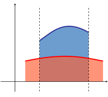Integral as area between two curves.

Double integral as volume under a surface z = x² − y². The rectangular region at the bottom of the body is the domain of integration, while the surface is the graph of the two-variable function to be integrated.

The multiple integral is a type of definite integral extended to functions of more than one real variable, for example, ƒ(x, y) or ƒ(x, y, z). Integrals of a function of two variables over a region in ℝ² are called double integrals.

Introduction

Just as the definite integral of a positive function of one variable represents the area of the region between the graph of the function and the x-axis, the double integral of a positive function of two variables represents the volume of the region between the surface defined by the function (on the three dimensional Cartesian plane where z = ƒ(x, y)) and the plane which contains its domain. (Note that the same volume can be obtained via the triple integral—the integral of a function in three variables—of the constant function ƒ(x, y, z) = 1 over the above-mentioned region between the surface and the plane.) If there are more variables, a multiple integral will yield hypervolumes of multi-dimensional functions.

Multiple integration of a function in n variables: f(x₁, x₂, ..., x_n) over a domain D is most commonly represented by nested integral signs in the reverse order of execution (the leftmost integral sign is computed last), followed by the function and integrand arguments in proper order (the integral with respect to the rightmost argument is computed last). The domain of integration is either represented symbolically for every argument over each integral sign, or is abbreviated by a variable at the rightmost integral sign:

$\int \cdots \int_\mathbf{D}\;f(x_1,x_2,\ldots,x_n) \;dx_1 \!\cdots dx_n$

Since the concept of an antiderivative is only defined for functions of a single real variable, the usual definition of the indefinite integral does not immediately extend to the multiple integral.

Mathematical definition

For n > 1, consider a so-called "half-open" n-dimensional hyperrectangular domain T, defined as:

$T=\left [ a_1, b_1 \right ) \times \left [ a_2, b_2 \right ) \times \cdots \times \left [ a_n, b_n \right ) \subseteq \mathbb R^n.$

Partition each interval [a_j, b_j) into a finite family I_j of non-overlapping subintervals i_jα , with each subinterval closed at the left end, and open at the right end.

Then the finite family of subrectangles C given by

$C=I_1\times I_2\times \cdots \times I_n$

is a partition of T; that is, the subrectangles C_k are non-overlapping and their union is T.

Let f : T → R be a function defined on T. Consider a partition C of T as defined above, such that C is a family of m subrectangles C_m and

$T=C_1\cup C_2\cup \cdots \cup C_m$

We can approximate the total nth-dimensional volume bounded below by T and above by f with the following Riemann sum:

$\sum_{k=1}^m f(P_k)\, \operatorname{m}(C_k)$

where P_k is a point in C_k and m(C_k) is the product of the lengths of the intervals whose Cartesian product is C_k, otherwise known as the measure of C_k.

The diameter of a subrectangle C_k is the largest of the lengths of the intervals whose Cartesian product is C_k. The diameter of a given partition of T is defined as the largest of the diameters of the subrectangles in the partition. Intuitively, as the diameter of the partition C is restricted smaller and smaller, the number of subrectangles m gets larger, and the measure m(C_k) of each subrectangle grows smaller. The function f is said to be Riemann integrable if the limit

$S=\lim_{\delta \to 0} \sum_{k=1}^m f(P_k)\, \operatorname{m}\, (C_k)$

exists, where the limit is taken over all possible partitions of T of diameter at most δ.

If f is Riemann integrable, S is called the Riemann integral of f over T and is denoted

$\int \cdots \int_T\;f(x_1,x_2,\ldots,x_n) \;dx_1 \!\cdots dx_n$

Frequently this notation is abbreviated as

$\int_T\!f(\mathbf{x})\,d\mathbf{x}.$

where x represents the n-tuple (x₁, ... x_n) and dx is the n-dimensional volume differential.

The Riemann integral of a function defined over an arbitrary bounded n-dimensional set can be defined by extending that function to a function defined over a half-open rectangle whose values are zero outside the domain of the original function. Then the integral of the original function over the original domain is defined to be the integral of the extended function over its rectangular domain, if it exists.

In what follows the Riemann integral in n dimensions will be called multiple integral.

Properties

Multiple integrals have many properties common to those of integrals of functions of one variable (linearity, commutativity, monotonicity, and so on.). One important property of multiple integrals is that the value of an integral is independent of the order of integrands under certain conditions. This property is popularly known as Fubini's theorem.

Particular cases

In the case of T ⊆ R², the integral

$\ell = \iint_T f(x,y)\, dx\, dy$

is the double integral of f on T, and if T ⊆ R³ the integral

$\ell = \iiint_T f(x,y,z)\, dx\, dy\, dz$

is the triple integral of f on T.

Notice that, by convention, the double integral has two integral signs, and the triple integral has three; this is a notational convention which is convenient when computing a multiple integral as an iterated integral, as shown later in this article.

Methods of integration

The resolution of problems with multiple integrals consists, in most of cases, of finding a way to reduce the multiple integral to an iterated integral, a series of integrals of one variable, each being directly solvable. Sometimes, it is possible to obtain the result of the integration by direct examination without any calculations.

Integrating constant functions

When the integrand is a constant function c, the integral is equal to the product of c and the measure of the domain of integration. If c = 1 and the domain is a subregion of R², the integral gives the area of the region, while if the domain is a subregion of R³, the integral gives the volume of the region.

• For example:

$D = \{ (x,y) \in \mathbb{R}^2 \ : \ 2 \le x \le 4 \ ; \ 3 \le y \le 6 \}$ and $f(x,y) = 2\,\!$

in which case

$\int_3^6 \int_2^4 \ 2 \ dx\, dy =2\int_3^6 \int_2^4 \ 1 \ dx\, dy= 2\cdot\mbox{area}(D) = (2 \cdot 3) \cdot 2 = 12$,

since $\int_3^6 \int_2^4 \ 1 \ dx\, dy=\mbox{area}(D)$ by definition.

Use of symmetry

When the domain of integration is symmetric about the origin with respect to at least one of the variables of integration and the integrand is odd with respect to this variable, the integral is equal to zero, as the integrals over the two halves of the domain have the same absolute value but opposite signs. When the integrand is even with respect to this variable, the integral is equal to twice the integral over one half of the domain, as the integrals over the two halves of the domain are equal.

• Example (1):

Consider the function f(x,y) = 2sinx − 3y³ + 5 integrated over the domain $T=\left \{ \left ( x,y \right ) \in R^2 | x^2+y^2\le 1 \right \}$, a disc with radius 1 centered at the origin with the boundary included.

Using the linearity property, the integral can be decomposed into three pieces:

$\iint_T (2\sin x - 3y^3 + 5) \, dx \, dy = \iint_T 2 \sin x \, dx \, dy - \iint_T 3y^3 \, dx \, dy + \iint_T 5 \, dx \, dy$

2  sin  x and 3y³ are both odd functions and moreover it is evident that the T disc has a symmetry for the x and even the y axis; therefore the only contribution to the final result of the integrals is that of the constant function 5 because the other two pieces are null.

• Example (2):

Consider the function f(x, y, z) = x exp(y² + z²) and as integration region the sphere with radius 2 centered at the origin of the axes T = x² + y² + z² ≤ 4. The "ball" is symmetric about all three axes, but it is sufficient to integrate with respect to x-axis to show that the integral is 0, because the function is an odd function of that variable.

Normal domains on R²

See also: Order of integration (calculus)

This method is applicable to any domain D for which:

• the projection of D onto either the x-axis or the y-axis is bounded by the two values, a and b
• any line perpendicular to this axis that passes between these two values intersects the domain in an interval whose endpoints are given by the graphs of two functions, α and β.

x-axis

If the domain D is normal with respect to the x-axis, and $f: D \longrightarrow \mathbb{R}$ is a continuous function; then α(x) and β(x) (defined on the interval [a, b]) are the two functions that determine D. Then:

$\iint_D f(x,y)\ dx\, dy = \int \limits_a^b dx \int \limits_{ \alpha (x)}^{ \beta (x)} f(x,y)\, dy.$

y-axis

If D is normal with respect to the y-axis and $f: D \longrightarrow \mathbb{R}$ is a continuous function; then α(y) and β(y) (defined on the interval [a, b]) are the two functions that determine D. Then:

$\iint_D f(x,y)\ dx\, dy = \int_a^b dy \int_{ \alpha (y)}^{ \beta (y)} f(x,y)\, dx.$

Example

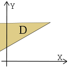
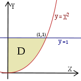Example: double integral over the normal region D

Consider this region: $D = \{ (x,y) \ \ x \ge 0, y \le 1, y \ge x^2 \}$ (please see the graphic in the example). Calculate

$\iint_D (x+y) \, dx \, dy.$

This domain is normal with respect to both the x- and y-axes. To apply the formulae it is required to find the functions that determine D and the intervals over which these are defined.

In this case the two functions are:

$\alpha (x) = x^2\text{ and }\beta (x) = 1\,\!$

while the interval is given by the intersections of the functions with x = 0, so the interval is [a, b] = [0, 1] (normality has been chosen with respect to the x-axis for a better visual understanding).

It is now possible to apply the formula:

$\iint_D (x+y) \, dx \, dy = \int_0^1 dx \int_{x^2}^1 (x+y) \, dy = \int_0^1 dx \ \left[xy \ + \ \frac{y^2}{2} \ \right]^1_{x^2}$

(at first the second integral is calculated considering x as a constant). The remaining operations consist of applying the basic techniques of integration:

$\int_0^1 \left[xy \ + \ \frac{y^2}{2} \ \right]^1_{x^2} \, dx = \int_0^1 \left(x + \frac{1}{2} - x^3 - \frac{x^4}{2} \right) dx = \cdots = \frac{13}{20}.$

If we choose normality with respect to the y-axis we could calculate

$\int_0^1 dy \int_0^{\sqrt{y}} (x+y) \, dx.$

and obtain the same value.

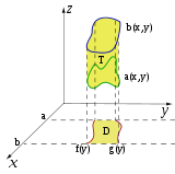Example of domain in R³ that is normal with respect to the xy-plane.

Normal domains on R³

The extension of these formulae to triple integrals should be apparent:

if T is a domain that is normal with respect to the xy-plane and determined by the functions α (x,y) and β(x,y), then

$\iiint_T f(x,y,z) \ dx\, dy\, dz = \iint_D \int_{\alpha (x,y)}^{\beta (x,y)} f(x,y,z) \, dz dx dy$

(this definition is the same for the other five normality cases on R³).

Change of variables

See also: Integration by substitution#Substitution for multiple variables

The limits of integration are often not easily interchangeable (without normality or with complex formulae to integrate). One makes a change of variables to rewrite the integral in a more "comfortable" region, which can be described in simpler formulae. To do so, the function must be adapted to the new coordinates.

Example (1-a):

The function is $f(x, y) = (x-1)^2 +\sqrt y$;

if one adopts this substitution $x' = x-1, \ y'= y \, \!$ therefore $x = x' + 1, \ y=y' \,\!$

one obtains the new function $f_2(x,y) = (x')^2 +\sqrt y$.

• Similarly for the domain because it is delimited by the original variables that were transformed before (x and y in example).
• the differentials dx and dy transform via the absolute value of the determinant of the Jacobian matrix containing the partial derivatives of the transformations regarding the new variable (consider, as an example, the differential transformation in polar coordinates).

There exist three main "kinds" of changes of variable (one in R², two in R³); however, more general substitutions can be made using the same principle.

Polar coordinates

See also: Polar coordinate system

Transformation from cartesian to polar coordinates.

In R² if the domain has a circular "symmetry" and the function has some "particular" characteristics you can apply the transformation to polar coordinates (see the example in the picture) which means that the generic points P(x,y) in Cartesian coordinates switch to their respective points in polar coordinates. That allows one to change the "shape" of the domain and simplify the operations.

The fundamental relation to make the transformation is the following:

$f(x,y) \rightarrow f(\rho \ \cos \phi,\rho \ \sin \phi ).$

Example (2-a):

The function is $f(x,y) = x + y\,\!$

and applying the transformation one obtains

$f(\rho, \phi) = \rho \cos \phi + \rho \sin \phi = \rho \ (\cos \phi + \sin \phi ).$

Example (2-b):

The function is $f(x,y) = x^2 + y^2\,\!$

In this case one has:

$f(\rho, \phi) = \rho^2 (\cos^2 \phi + \sin^2 \phi) = \rho^2\,\!$

using the Pythagorean trigonometric identity (very useful to simplify this operation).

The transformation of the domain is made by defining the radius' crown length and the amplitude of the described angle to define the ρ, φ intervals starting from x, y.

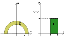Example of a domain transformation from cartesian to polar.

Example (2-c):

The domain is $D = x^2 + y^2 \le 4\,\!$, that is a circumference of radius 2; it's evident that the covered angle is the circle angle, so φ varies from 0 to 2π, while the crown radius varies from 0 to 2 (the crown with the inside radius null is just a circle).

Example (2-d):

The domain is $D = \{ x^2 + y^2 \le 9, \ x^2 + y^2 \ge 4, \ y \ge 0 \}$, that is the circular crown in the positive y half-plane (please see the picture in the example); note that φ describes a plane angle while ρ varies from 2 to 3. Therefore the transformed domain will be the following rectangle:

$T = \{ 2 \le \rho \le 3, \ 0 \le \phi \le \pi \}. \,$

The Jacobian determinant of that transformation is the following:

$\frac{\partial (x,y)}{\partial (\rho, \phi)} = \begin{vmatrix} \cos \phi & - \rho \sin \phi \\ \sin \phi & \rho \cos \phi \end{vmatrix} = \rho$

which has been obtained by inserting the partial derivatives of x = ρ cos(φ), y = ρ sin(φ) in the first column respect to ρ and in the second respect to φ, so the dx dy differentials in this transformation becomes ρ dρ dφ.

Once the function is transformed and the domain evaluated, it is possible to define the formula for the change of variables in polar coordinates:

$\iint_D f(x,y) \ dx\, dy = \iint_T f(\rho \cos \phi, \rho \sin \phi) \rho \, d \rho\, d \phi.$

Please note that φ is valid in the [0, 2π] interval while ρ, which is a measure of a length, can only have positive values.

Example (2-e):

The function is ƒ(x, y) = x and as the domain the same in 2-d example.

From the previous analysis of D we know the intervals of ρ (from 2 to 3) and of φ (from 0 to π). Now let's change the function:

$f(x,y) = x \longrightarrow f(\rho,\phi) = \rho \ \cos \phi.\,$

finally let's apply the integration formula:

$\iint_D x \, dx\, dy = \iint_T \rho \cos \phi \ \rho \, d\rho\, d\phi.$

Once the intervals are known, you have

$\int_0^\pi \int_2^3 \rho^2 \cos \phi \ d \rho \ d \phi = \int_0^\pi \cos \phi \ d \phi \left[ \frac{\rho^3}{3} \right]_2^3 = \left[ \sin \phi \right]_0^\pi \ \left(9 - \frac{8}{3} \right) = 0.$

Cylindrical coordinates

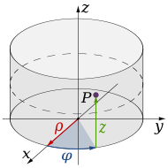Cylindrical coordinates.

In R³ the integration on domains with a circular base can be made by the passage in cylindrical coordinates; the transformation of the function is made by the following relation:

$f(x,y,z) \rightarrow f(\rho \ \cos \phi,\rho \ \sin \phi, z)$

The domain transformation can be graphically attained, because only the shape of the base varies, while the height follows the shape of the starting region.

Example (3-a):

The region is $D = \{ x^2 + y^2 \le 9, \ x^2 + y^2 \ge 4, \ 0 \le z \le 5 \}$ (that is the "tube" whose base is the circular crown of the 2-d example and whose height is 5); if the transformation is applied, this region is obtained: $T = \{ 2 \le \rho \le 3, \ 0 \le \phi \le 2\pi, \ 0 \le z \le 5 \}$ (that is the parallelepiped whose base is similar to the rectangle in 2-d example and whose height is 5).

Because the z component is unvaried during the transformation, the dx dy dz differentials vary as in the passage in polar coordinates: therefore, they become ρ dρ dφ dz.

Finally, it is possible to apply the final formula to cylindrical coordinates:

$\iiint_D f(x,y,z) \, dx\, dy\, dz = \iiint_T f(\rho \cos \phi, \rho \sin \phi, z) \rho \, d\rho\, d\phi\, dz.$

This method is convenient in case of cylindrical or conical domains or in regions where it is easy to individuate the z interval and even transform the circular base and the function.

Example (3-b):

The function is $f(x,y,z) = x^2 + y^2 + z\,\!$ and as integration domain this cylinder: $D = \{ x^2 + y^2 \le 9, \ -5 \le z \le 5 \}$.

The transformation of D in cylindrical coordinates is the following:

$T = \{ 0 \le \rho \le 3, \ 0 \le \phi \le 2 \pi, \ -5 \le z \le 5 \}.$

while the function becomes

$f(\rho \ \cos \phi,\rho \ \sin \phi, z) = \rho^2 + z\,\!$

Finally one can apply the integration formula:

$\iiint_D (x^2 + y^2 +z) \, dx\, dy\, dz = \iiint_T ( \rho^2 + z) \rho \, d\rho\, d\phi\, dz;$

developing the formula you have

$\int_{-5}^5 dz \int_0^{2 \pi} d\phi \int_0^3 ( \rho^3 + \rho z )\, d\rho = 2 \pi \int_{-5}^5 \left[ \frac{\rho^4}{4} + \frac{\rho^2 z}{2} \right]_0^3 \, dz$

$= 2 \pi \int_{-5}^5 \left( \frac{81}{4} + \frac{9}{2} z\right)\, dz = \cdots = 405 \pi.$

Spherical coordinates

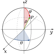Spherical coordinates.

In R³ some domains have a spherical symmetry, so it's possible to specify the coordinates of every point of the integration region by two angles and one distance. It's possible to use therefore the passage in spherical coordinates; the function is transformed by this relation:

$f(x,y,z) \longrightarrow f(\rho \cos \theta \sin \phi, \rho \sin \theta \sin \phi, \rho \cos \phi)\,\!$

Note that points on z axis do not have a precise characterization in spherical coordinates, so θ can vary between 0 to 2π .

The better integration domain for this passage is obviously the sphere.

Example (4-a):

The domain is $D = x^2 + y^2 + z^2 \le 16$ (sphere with radius 4 and center in the origin); applying the transformation you get this region: $T = \{ 0 \le \rho \le 4, \ 0 \le \phi \le \pi, \ 0 \le \theta \le 2 \pi \}.$

The Jacobian determinant of this transformation is the following:

$\frac{\partial (x,y,z)}{\partial (\rho, \theta, \phi)} = \begin{vmatrix} \cos \theta \sin \phi & - \rho \sin \theta \sin \phi & \rho \cos \theta \cos \phi \\ \sin \theta \sin \phi & \rho \cos \theta \sin \phi & \rho \sin \theta \cos \phi \\ \cos \phi & 0 & - \rho \sin \phi \end{vmatrix} = \ \rho^2 \sin \phi$

The dx dy dz differentials therefore are transformed to ρ² sin(φ) dρ dθ dφ.

Finally you obtain the final integration formula:

$\iiint_D f(x,y,z) \, dx\, dy\, dz = \iiint_T f(\rho \sin \phi \cos \theta, \rho \sin \phi \sin \theta, \rho \cos \phi) \rho^2 \sin \phi \, d\rho\, d\theta\, d\phi.$

It's better to use this method in case of spherical domains and in case of functions that can be easily simplified, by the first fundamental relation of trigonometry, extended in R³ (please see example 4-b); in other cases it can be better to use cylindrical coordinates (please see example 4-c).

$\iiint_T f(a,b,c) \rho^2 \sin \phi \, d\rho\, d\theta\, d\phi.$

Note that the extra ρ² and sin ϕ come from the Jacobian.

Note that in the following examples the roles of φ and θ have been reversed.

Example (4-b):

D is the same region of the 4-a example and $f(x,y,z) = x^2 + y^2 + z^2\,\!$ is the function to integrate.

Its transformation is very easy:

$f(\rho \sin \phi \cos \theta, \rho \sin \phi \sin \theta, \rho \cos \phi) = \rho^2,\,$

while we know the intervals of the transformed region T from D:

$(0 \le \rho \le 4, \ 0 \le \phi \le \pi, \ 0 \le \theta \le 2 \pi).\,$

Let's therefore apply the integration's formula:

$\iiint_D (x^2 + y^2 +z^2) \, dx\, dy\, dz = \iiint_T \rho^2 \ \rho^2 \sin \theta \, d\rho\, d\theta\, d\phi,$

and, developing, we get

$\iiint_T \rho^4 \sin \theta \, d\rho\, d\theta\, d\phi = \int_0^{\pi} \sin \phi \,d\phi \int_0^4 \rho^4 d \rho \int_0^{2 \pi} d\theta = 2 \pi \int_0^{\pi} \sin \phi \left[ \frac{\rho^5}{5} \right]_0^4 \, d \phi$

$= 2 \pi \left[ \frac{\rho^5}{5} \right]_0^4 \left[- \cos \phi \right]_0^{\pi} = 4 \pi \cdot \frac{1024}{5} = \frac{4096 \pi}{5}.$

Example (4-c):

The domain D is the ball with center in the origin and radius 3a ($D = x^2 + y^2 + z^2 \le 9a^2 \,\!$) and $f(x,y,z) = x^2 + y^2\,\!$ is the function to integrate.

Looking at the domain, it seems convenient to adopt the passage in spherical coordinates, in fact, the intervals of the variables that delimit the new T region are obviously:

$0 \le \rho \le 3a, \ 0 \le \phi \le 2 \pi, \ 0 \le \theta \le \pi.\,$

However, applying the transformation, we get

$f(x,y,z) = x^2 + y^2 \longrightarrow \rho^2 \sin^2 \theta \cos^2 \phi + \rho^2 \sin^2 \theta \sin^2 \phi = \rho^2 \sin^2 \theta$.

Applying the formula for integration we would obtain:

$\iiint_T \rho^2 \sin^2 \theta \rho^2 \sin \theta \, d\rho\, d\theta\, d\phi = \iiint_T \rho^4 \sin^3 \theta \, d\rho\, d\theta\, d\phi$

which is very hard to solve. This problem will be solved by using the passage in cylindrical coordinates. The new T intervals are

$0 \le \rho \le 3a, \ 0 \le \phi \le 2 \pi, \ - \sqrt{9a^2 - \rho^2} \le z \le \sqrt{9a^2 - \rho^2};$

the z interval has been obtained by dividing the ball in two hemispheres simply by solving the inequality from the formula of D (and then directly transforming x² + y² in ρ²). The new function is simply ρ². Applying the integration formula

$\iiint_T \rho^2 \rho \ d \rho d \phi dz$.

Then we get

$\int_0^{2 \pi} d\phi \int_0^{3a} \rho^3 d\rho \int_{- \sqrt{9a^2 - \rho^2} }^{\sqrt{9 a^2 - \rho^2} }\, dz = 2 \pi \int_0^{3a} 2 \rho^3 \sqrt{9 a^2 - \rho^2} \, d\rho.$

Now let's apply the transformation

$9 a^2 - \rho^2 = t\,\! \longrightarrow dt = -2 \rho\, d\rho \longrightarrow d\rho = \frac{d t}{- 2 \rho}\,\!$

(the new intervals become $0, 3a \longrightarrow 9 a^2, 0$). We get

$- 2 \pi \int_{9 a^2}^{0} \rho^2 \sqrt{t}\, dt$

because $\rho^2 = 9 a^2 - t\,\!$, we get

$-2 \pi \int_{9 a^2}^0 (9 a^2 - t) \sqrt{t}\, dt,$

after inverting the integration's bounds and multiplying the terms between parenthesis, it is possible to decompose the integral in two parts that can be directly solved:

$2 \pi \left[ \int_0^{9 a^2} 9 a^2 \sqrt{t} \, dt - \int_0^{9 a^2} t \sqrt{t} \, dt\right] = 2 \pi \left[9 a^2 \frac{2}{3} t^{ \frac{3}{2} } - \frac{2}{5} t^{ \frac{5}{2}} \right]_0^{9 a^2}$

$= 2 \cdot 27 \pi a^5 ( 6 - \frac{2}{5} ) = 54 \pi \frac{28}{5} a^5 = \frac{1512 \pi}{5} a^5.$

Thanks to the passage in cylindrical coordinates it was possible to reduce the triple integral to an easier one-variable integral.

See also the differential volume entry in nabla in cylindrical and spherical coordinates.

Examples

Double integral

Let us assume that we wish to integrate a multivariable function f over a region A.

$A = \{ (x,y) \in \mathbb{R}^2 \ : \ 11 \le x \le 14 \ ; \ 7 \le y \le 10 \}\text{ and }f(x,y) = x^2 + 4y\,$

From this we formulate the double integral

$\int_7^{10} \int_{11}^{14} \ (x^2 + 4y) \ dx\, dy$

The inner integral is performed first, integrating with respect to x and taking y as a constant, as it is not the variable of integration. The result of this integral, which is a function depending only on y, is then integrated with respect to y.

$\begin{align} \int_{11}^{14} \ (x^2 \ + \ 4y) \ dx & = \left (\frac{1}{3}x^3 \ + \ 4yx \right)\Big |_{x=11}^{x=14} \\ & = \frac{1}{3}(14)^3 \ + \ 4y(14) \ - \ \frac{1}{3}(11)^3 \ - \ 4y(11) \\ &= 471 \ + \ 12y \end{align}$

We then integrate the result with respect to y.

$\begin{align} \int_7^{10} \ (471 \ + \ 12y) \ dy & = (471y\ + \ 6y^2)\big |_{y=7}^{y=10} \\ & = 471(10) \ + \ 6(10)^2 \ - \ 471(7) \ - \ 6(7)^2 \\ &= 1719 \end{align}$

Volumes

The volume of the parallelepiped of sides 4 × 6 × 5 may be obtained in two ways:

• By calculating the double integral of the function f(x, y) = 5 over the region D in the xy-plane which is the base of the parallelepiped.

$\iint_D 5 \ dx\, dy$

• By calculating the triple integral of the constant function 1 over the parallelepiped itself

$\iiint_\mathrm{parallelepiped} 1 \, dx\, dy\, dz$

Computing a volume

Using the methods previously described, it is possible to calculate the volumes of some common solids.

• Cylinder: The volume of a cylinder with height h and circular base of radius R can be calculated by integrating the constant function h over the circular base, using polar coordinates.

$\mathrm{Volume} = \int_0^{2 \pi } d \phi \int_0^R h \rho \ d \rho = h 2 \pi \left[\frac{\rho^2}{2 }\right]_0^R = \pi R^2 h$

This is in agreement with the formula

$\mathrm{Volume} = \text{base area} \times i R^2 h$.

• Sphere: The volume of a sphere with radius R can be calculated by integrating the constant function 1 over the sphere, using spherical coordinates.

$\text{Volume} = \iiint_D f(x,y,z) \, dx\, dy\, dz = \iiint_D 1 \, dV = \iiint_S \rho^2 \sin \phi \, d\rho\, d\theta\, d\phi$

$= \int_0^{2 \pi }\, d \theta \int_0^{ \pi } \sin \phi\, d \phi \int_0^R \rho^2\, d \rho = 2 \pi \int_0^{ \pi } \sin \phi\, d \phi \int_0^R \rho^2\, d \rho= 2 \pi \int_0^{ \pi } \sin \phi \frac{R^3}{3 }\, d \phi = \frac{2}{3 } \pi R^3 [- \cos \phi]_0^{ \pi } = \frac{4}{3 } \pi R^3.$

• Tetrahedron (triangular pyramid or 3-simplex): The volume of a tetrahedron with its apex at the origin and edges of length l along the x, y and z axes can be calculated by integrating the constant function 1 over the tetrahedron.

$\text{Volume} = \int_0^\ell dx \int_0^{\ell-x }\, dy \int_0^{\ell-x-y }\, dz = \int_0^\ell dx \int_0^{\ell-x } (\ell - x - y)\, dy$

$= \int_0^\ell \left[\ell^2 - 2\ell x + x^2 - \frac{ (\ell-x)^2 }{2 }\right]\, dx = \ell^3 - \ell \ell^2 + \frac{\ell^3}{3 } - \left[\frac{\ell^2}{2 } - \ell x + \frac{x^2}{2 }\right]_0^\ell$

$= \frac{\ell^3}{3 } - \frac{\ell^3}{6 } = \frac{\ell^3}{6}$

This is in agreement with the formula

$\mathrm{Volume} = \frac{1}{3} \times \text{base area} \times \text{height} = \frac{1}{3} \times \frac{\ell^2}{2} \times \ell = \frac{\ell^3}{6}$.

Example of an improper domain.

Multiple improper integral

In case of unbounded domains or functions not bounded near the boundary of the domain, we have to introduce the double improper integral or the triple improper integral.

Multiple integrals and iterated integrals

See also: Order of integration (calculus)

Fubini's theorem states that if

$\int_{A\times B} |f(x,y)|\,d(x,y)<\infty,$

that is, if the integral is absolutely convergent, then the multiple integral will give the same result as the iterated integral,

$\int_{A\times B} f(x,y)\,d(x,y)=\int_A\left(\int_B f(x,y)\,dy\right)\,dx=\int_B\left(\int_A f(x,y)\,dx\right)\,dy.$

In particular this will occur if |f(x,y)| is a bounded function and A and B are bounded sets.

If the integral is not absolutely convergent, care is needed not to confuse the concepts of multiple integral and iterated integral, especially since the same notation is often used for either concept. The notation

$\int_0^1\int_0^1 f(x,y)\,dy\,dx$

means, in some cases, an iterated integral rather than a true double integral. In an iterated integral, the outer integral

$\int_0^1 \cdots \, dx$

is the integral with respect to x of the following function of x:

$g(x)=\int_0^1 f(x,y)\,dy.$

A double integral, on the other hand, is defined with respect to area in the xy-plane. If the double integral exists, then it is equal to each of the two iterated integrals (either "dy dx" or "dx dy") and one often computes it by computing either of the iterated integrals. But sometimes the two iterated integrals exist when the double integral does not, and in some such cases the two iterated integrals are different numbers, i.e., one has

$\int_0^1\int_0^1 f(x,y)\,dy\,dx \neq \int_0^1\int_0^1 f(x,y)\,dx\,dy.$

This is an instance of rearrangement of a conditionally convergent integral.

The notation

$\int_{[0,1]\times[0,1]} f(x,y)\,dx\,dy$

may be used if one wishes to be emphatic about intending a double integral rather than an iterated integral.

Some practical applications

Quite generally, just as in one variable, one can use the multiple integral to find the average of a function over a given set. Given a set D ⊆ Rⁿ and an integrable function f over D, the average value of f over its domain is given by

$\bar{f} = \frac{1}{m(D)} \int_D f(x)\, dx,$

where m(D) is the measure of D.

Additionally, multiple integrals are used in many applications in physics. The examples below also show some variations in the notation.

In mechanics, the moment of inertia is calculated as the volume integral (triple integral) of the density weighed with the square of the distance from the axis:

$I_z = \iiint_V \rho r^2\, dV.$

The gravitational potential associated with a mass distribution given by a mass measure dm on three-dimensional Euclidean space R³ is

$V(\mathbf{x}) = -\int_{\mathbf{R}^3} \frac{G}{|\mathbf{x} - \mathbf{y}|}\,dm(\mathbf{y}).$

If there is a continuous function ρ(x) representing the density of the distribution at x, so that dm(x) = ρ(x)d³x, where d³x is the Euclidean volume element, then the gravitational potential is

$V(\mathbf{x}) = -\int_{\mathbf{R}^3} \frac{G}{|\mathbf{x}-\mathbf{y}|}\,\rho(\mathbf{y})\,d^3\mathbf{y}.$

In electromagnetism, Maxwell's equations can be written using multiple integrals to calculate the total magnetic and electric fields. In the following example, the electric field produced by a distribution of charges given by the volume charge density $\rho (\vec r)$ is obtained by a triple integral of a vector function:

$\vec E = \frac {1}{4 \pi \epsilon_0} \iiint \frac {\vec r - \vec r'}{\left \| \vec r - \vec r' \right \|^3} \rho (\vec r')\, \operatorname{d}^3 r'.$

This can also be written as an integral with respect to a signed measure representing the charge distribution.

See also

• Main analysis theorems that relate multiple integrals:
  • Divergence theorem
  • Stokes' theorem
  • Green's theorem

Free software for multidimensional numerical integration

• interalg: a solver from OpenOpt/FuncDesigner frameworks, based on interval analysis, guaranteed precision, license: BSD (free for any purposes)
• Cuba is a free-software library of several multi-dimensional integration algorithms
• Cubature code for adaptive multi-dimensional integration

References

• Robert A. Adams - Calculus: A Complete Course (5th Edition) ISBN 0201791315.
• R.K.Jain and S.R.K Iyengar- Advanced Engineering Mathematics (Third edition) 2009, Narosa Publishing House ISBN 9788173197307

External links

• Weisstein, Eric W., "Multiple Integral" from MathWorld.
• L.D. Kudryavtsev (2001), "Multiple integral", in Hazewinkel, Michiel, Encyclopaedia of Mathematics, Springer, ISBN 978-1556080104, http://eom.springer.de/M/m065370.htm 
• Mathematical Assistant on Web online evaluation of double integrals in Cartesian coordinates and polar coordinates (includes intermediate steps in the solution, powered by Maxima (software))