Potential flow

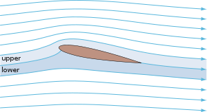Potential-flow streamlines around a NACA 0012 airfoil at 11° angle of attack, with upper and lower streamtubes identified.

In fluid dynamics, potential flow describes the velocity field as the gradient of a scalar function: the velocity potential. As a result, a potential flow is characterized by an irrotational velocity field, which is a valid approximation for several applications. The irrotationality of a potential flow is due to the curl of a gradient always being equal to zero.

In the case of an incompressible flow the velocity potential satisfies Laplace's equation, and potential theory is applicable. However, potential flows also have been used to describe compressible flows. The potential flow approach occurs in the modeling of both stationary as well as nonstationary flows.

Applications of potential flow are for instance: the outer flow field for aerofoils, water waves, electroosmotic flow, and groundwater flow. For flows (or parts thereof) with strong vorticity effects, the potential flow approximation is not applicable.

Characteristics and applications

A potential flow is constructed by adding simple elementary flows and observing the result.

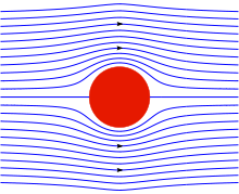Streamlines for the incompressible potential flow around a circular cylinder in a uniform onflow.

Description and characteristics

In fluid dynamics, a potential flow is described by means of a velocity potential φ, being a function of space and time. The flow velocity v is a vector field equal to the gradient, ∇, of the velocity potential φ:^[1]

$\mathbf{v} = \nabla \varphi.$

Sometimes, also the definition v = −∇φ, with a minus sign, is used. But here we will use the definition above, without the minus sign. From vector calculus it is known, that the curl of a gradient is equal to zero:^[1]

$\nabla \times \nabla \varphi = \mathbf{0},$

and consequently the vorticity, the curl of the velocity field v, is zero:^[1]

$\nabla \times \mathbf{v} = \mathbf{0}.$

This implies that a potential flow is an irrotational flow. This has direct consequences for the applicability of potential flow. In flow regions where vorticity is known to be important, such as wakes and boundary layers, potential flow theory is not able to provide reasonable predictions of the flow.^[2] Fortunately, there are often large regions of a flow where the assumption of irrotationality is valid, which is why potential flow is used for various applications. For instance in: flow around aircraft, groundwater flow, acoustics, water waves, and electroosmotic flow.^[3]

Incompressible flow

In case of an incompressible flow — for instance of a liquid, or a gas at low Mach numbers; but not for sound waves — the velocity v has zero divergence:^[1]

$\nabla \cdot \mathbf{v} =0,$

with the dot denoting the inner product. As a result, the velocity potential φ has to satisfy Laplace's equation^[1]

$\nabla^2 \varphi = 0,$

where $\nabla^2 = \nabla \cdot \nabla$ is the Laplace operator (sometimes also written Δ). In this case the flow can be determined completely from its kinematics: the assumptions of irrotationality and zero divergence of the flow. Dynamics only have to be applied afterwards, if one is interested in computing pressures: for instance for flow around airfoils through the use of Bernoulli's principle.

In two dimensions, potential flow reduces to a very simple system that is analyzed using complex analysis (see below).

Compressible flow

Steady flow

Potential flow theory can also be used to model irrotational compressible flow. The full potential equation, describing a steady flow, is given by:^[4]

$\begin{align} & \left( 1 - M_x^2 \right) \frac{\partial^2 \Phi}{\partial x^2} + \left( 1 - M_y^2 \right) \frac{\partial^2 \Phi}{\partial y^2} + \left( 1 - M_z^2 \right) \frac{\partial^2 \Phi}{\partial z^2} \\ & \quad - 2 M_x M_y \frac{\partial^2 \Phi}{\partial x\, \partial y} - 2 M_y M_z \frac{\partial^2 \Phi}{\partial y\, \partial z} - 2 M_z M_x \frac{\partial^2 \Phi}{\partial z\, \partial x} = 0, \end{align}$

with Mach number components

$M_x = \frac{1}{a} \frac{\partial \Phi}{\partial x},$   $M_y = \frac{1}{a} \frac{\partial \Phi}{\partial y}$   and   $M_z = \frac{1}{a} \frac{\partial \Phi}{\partial z},$  

where a is the local speed of sound. The flow velocity v is again equal to ∇Φ, with Φ the velocity potential. The full potential equation is valid for sub-, trans- and supersonic flow at arbitrary angle of attack, as long as the assumption of irrotationality is applicable.^[4]

In case of either subsonic or supersonic (but not transsonic or hypersonic) flow, at small angles of attack and thin bodies, an additional assumption can be made: the velocity potential is split into an undisturbed onflow velocity V_∞ in the x-direction, and small a perturbation velocity ∇φ thereof. So:^[4]

$\nabla \Phi = V_\infty x + \nabla \varphi.$

In that case, the linearized small-perturbation potential equation — an approximation to the full potential equation — can be used:^[4]

$\left(1-M_\infty^2\right) \frac{\partial^2 \varphi}{\partial x^2} + \frac{\partial^2 \varphi}{\partial y^2} + \frac{\partial^2 \varphi}{\partial z^2} = 0,$

with M_∞ = V_∞ / a_∞ the Mach number of the incoming free stream. This linear equation is much easier to solve than the full potential equation: it may be recast into Laplace's equation by a simple coordinate stretching in the x-direction.

Derivation of the full potential equation

For a steady inviscid flow, the Euler equations — for the mass and momentum density — are, in subscript notation and in non-conservation form:[5] $\begin{align} \frac{\partial}{\partial x_i} \left( \rho\, v_i \right) &= 0, \\ \rho\, v_j\, \frac{\partial v_i}{\partial x_j} &= - \frac{\partial p}{\partial x_i}, \end{align}$ while using the summation convention: since j occurs more than once in the term on the left hand side of the momentum equation, j is summed over all its components (which is from j=1 to 2 in two-dimensional flow, and from j=1 to 3 in three dimensions). Further: ρ is the fluid density, p is the pressure, (x1,x2,x3) = (x,y,z) are the coordinates and (v1,v2,v3) are the corresponding components of the velocity vector v. The speed of sound squared a2 is equal to the derivative of the pressure p with respect to the density ρ, at constant entropy S:[6] $a^2 = \left[ \frac{\partial p}{\partial \rho} \right]_S.$ As a result, the flow equations can be written as: $v_i\, \frac{\partial \rho}{\partial x_i} + \rho\, \frac{\partial v_i}{\partial x_i} = 0$   and   $\rho\, v_j\, \frac{\partial v_i}{\partial x_j} = -a^2\, \frac{\partial \rho}{\partial x_i}.$ Multiplying (and summing) the momentum equation with vi, and using the mass equation to eliminate the density gradient gives: $\rho\, v_i\, v_j\, \frac{\partial v_i}{\partial x_j} = \rho\, a^2\, \frac{\partial v_i}{\partial x_i}.$ When divided by ρ, and with all terms on one side of the equation, the compressible flow equation is: $\frac{\partial v_i}{\partial x_i} - \frac{v_i\, v_j}{a^2} \frac{\partial v_i}{\partial x_j} = 0.$ Note that until this stage, no assumptions have been made regarding the flow (besides that it is a steady flow). Now, for irrotational flow the velocity v is the gradient of the velocity potential Φ, and the local Mach number components Mi are defined as: $v_i = \frac{\partial \Phi}{\partial x_i}$   and   $M_i = \frac{v_i}{a} = \frac{1}{a} \frac{\partial \Phi}{\partial x_i}.$ When used in the flow equation, the full potential equation results: $\frac{\partial^2 \Phi}{\partial x_i\, \partial x_i} - M_i\, M_j\, \frac{\partial^2 \Phi}{\partial x_i\, \partial x_j} = 0.$ Written out in components, the form given at the beginning of this section is obtained. When a specific equation of state is provided, relating pressure p and density ρ, the speed of sound can be determined. Subsequently, together with adequate boundary conditions, the full potential equation can be solved (most often through the use of a computational fluid dynamics code).

Sound waves

Main articles: Sound, Acoustics, and Wave equation

Small-amplitude sound waves can be approximated with the following potential-flow model:^[7]

$\frac{\partial^2 \varphi}{\partial t^2} = \overline{a}^2 \Delta \varphi,$

which is a linear wave equation for the velocity potential φ. Again the oscillatory part of the velocity vector v is related to the velocity potential by v = ∇φ, while as before Δ is the Laplace operator, and ā is the average speed of sound in the homogeneous medium. Note that also the oscillatory parts of the pressure p and density ρ each individually satisfy the wave equation, in this approximation.

Applicability and limitations

Potential flow does not include all the characteristics of flows that are encountered in the real world. For example, potential flow excludes turbulence, which is commonly encountered in nature. Also, potential flow theory cannot be applied for viscous internal flows.^[2] Richard Feynman considered potential flow to be so unphysical that the only fluid to obey the assumptions was "dry water".^[8]

Incompressible potential flow also makes a number of invalid predictions, such as d'Alembert's paradox, which states that the drag on any object moving through an infinite fluid otherwise at rest is zero.^[9]

More precisely, potential flow cannot account for the behaviour of flows that include a boundary layer.^[2]

Nevertheless, understanding potential flow is important in many branches of fluid mechanics. In particular, simple potential flows (called elementary flows) such as the free vortex and the point source possess ready analytical solutions. These solutions can be superposed to create more complex flows satisfying a variety of boundary conditions. These flows correspond closely to real-life flows over the whole of fluid mechanics; in addition, many valuable insights arise when considering the deviation (often slight) between an observed flow and the corresponding potential flow.

Potential flow finds many applications in fields such as aircraft design. For instance, in computational fluid dynamics, one technique is to couple a potential flow solution outside the boundary layer to a solution of the boundary layer equations inside the boundary layer.

The absence of boundary layer effects means that any streamline can be replaced by a solid boundary with no change in the flow field, a technique used in many aerodynamic design approaches. Another technique would be the use of Riabouchinsky solids.^{[dubious – discuss]}

Analysis for two-dimensional flow

Main article: Conformal mapping

Potential flow in two dimensions is simple to analyze using conformal mapping, by the use of transformations of the complex plane. However, use of complex numbers is not required, as for example in the classical analysis of fluid flow past a cylinder. It is not possible to solve a potential flow using complex numbers in three dimensions.^[10]

The basic idea is to use a holomorphic (also called analytic) or meromorphic function f, which maps the physical domain (x,y) to the transformed domain (φ,ψ). While x, y, φ and ψ are all real valued, it is convenient to define the complex quantities

$z=x+iy\,$   and   $w=\varphi+i\psi.\,$

Now, if we write the mapping f as^[10]

$f(x+iy)=\varphi+i\psi\,$   or   $f(z)=w.\,$

Then, because f is a holomorphic or meromorphic function, it has to satisfy the Cauchy-Riemann equations^[10]

$\frac{\partial\varphi}{\partial x}=\frac{\partial\psi}{\partial y}, \qquad \frac{\partial\varphi}{\partial y}=-\frac{\partial\psi}{\partial x}.$

The velocity components (u,v), in the (x,y) directions respectively, can be obtained directly from f by differentiating with respect to z. That is^[10]

$\frac{df}{dz}=u-iv$

So the velocity field v = (u,v) is specified by^[10]

$u=\frac{\partial\varphi}{\partial x}=\frac{\partial\psi}{\partial y},\qquad v=\frac{\partial\varphi}{\partial y}=-\frac{\partial\psi}{\partial x}.$

Both φ and ψ then satisfy Laplace's equation:^[10]

$\Delta\varphi = \frac{\partial^2\varphi}{\partial x^2} + \frac{\partial^2\varphi}{\partial y^2} = 0$   and   $\Delta\psi = \frac{\partial^2\psi}{\partial x^2} + \frac{\partial^2\psi}{\partial y^2} = 0.$

So φ can be identified as the velocity potential and ψ is called the stream function.^[10] Lines of constant ψ are known as streamlines and lines of constant φ are known as equipotential lines (see equipotential surface).

Streamlines and equipotential lines are orthogonal to each other, since^[10]

$\nabla \phi \cdot \nabla \psi = \frac{\partial\phi}{\partial x}\frac{\partial\psi}{\partial x}+ \frac{\partial\phi}{\partial y}\frac{\partial\psi}{\partial y}= {\partial \psi \over \partial y} {\partial \psi \over \partial x} - {\partial \psi \over \partial x} {\partial \psi \over \partial y} = 0.$

Thus the flow occurs along the lines of constant ψ and at right angles to the lines of constant φ.^[10]

It is interesting to note that Δψ = 0 is also satisfied, this relation being equivalent to ∇×v = 0. So the flow is irrotational. The automatic condition ∂²Ψ /( ∂x ∂y) = ∂²Ψ /( ∂y ∂x) then gives the incompressibility constraint ∇·v = 0.

Examples of two-dimensional potential flows

General considerations

Any differentiable function may be used for f. The examples that follow use a variety of elementary functions; special functions may also be used.

Note that multi-valued functions such as the natural logarithm may be used, but attention must be confined to a single Riemann surface.

Power laws

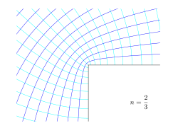
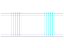
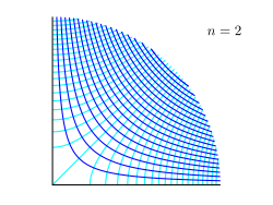
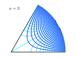
Examples of conformal maps for the power law w = A zn, for different values of the power n. Shown is the z-plane, showing lines of constant potential φ and streamfunction ψ, while w = φ + iψ.

In case the following power-law conformal map is applied, from z = x+iy to w = φ+iψ:^[11]

$w=Az^n, \,$

then, writing z in polar coordinates as z = x + iy = re^iθ, we have^[11]

$\varphi=Ar^n\cos n\theta\,$   and   $\psi=Ar^n\sin n\theta.\,$

In the figures to the right examples are given for several values of n. The black line is the boundary of the flow, while the darker blue lines are streamlines, and the lighter blue lines are equi-potential lines. Some interesting powers n are:^[11]

• n = ½ : this corresponds with flow around a semi-infinite plate,
• n = ⅔ : flow around a right corner,
• n = 1 : a trivial case of uniform flow,
• n = 2 : flow through a corner, or near a stagnation point, and
• n = -1 : flow due to a source doublet

The constant A is a scaling parameter: its absolute value |A| determines the scale, while its argument arg{A} introduces a rotation (if non-zero).

Power laws with n = 1: uniform flow

If w = Az¹, that is, a power law with n = 1, the streamlines (i.e. lines of constant ψ) are a system of straight lines parallel to the x-axis. This is easiest to see by writing in terms of real and imaginary components:

$f(x+iy)=A\times(x+iy)=Ax+i\cdot Ay$

thus giving φ = Ax and ψ = Ay. This flow may be interpreted as uniform flow parallel to the x-axis.

Power laws with n = 2

If n = 2, then w = Az² and the streamline corresponding to a particular value of ψ are those points satisfying

$\psi=Ar^2\sin 2\theta,\,$

which is a system of rectangular hyperbolae. This may be seen by again rewriting in terms of real and imaginary components. Noting that $\sin 2\theta=2\sin\theta\,\cos\theta$ and rewriting sin θ = y / r and cos θ = x / r it is seen (on simplifying) that the streamlines are given by

$\psi=2Axy.\,$

The velocity field is given by $\nabla\varphi$, or

$\begin{pmatrix} u \\ v \end{pmatrix} = \begin{pmatrix} \displaystyle {\partial \varphi \over \partial x} \\[2ex] \displaystyle {\partial \varphi \over \partial y} \end{pmatrix} = \begin{pmatrix} \displaystyle + {\partial \psi \over \partial y} \\[2ex] \displaystyle - {\partial \psi \over \partial x} \end{pmatrix} = \begin{pmatrix} +2Ax \\[2ex] -2Ay \end{pmatrix}.$

In fluid dynamics, the flowfield near the origin corresponds to a stagnation point. Note that the fluid at the origin is at rest (this follows on differentiation of f(z) = z² at z = 0).

The ψ = 0 streamline is particularly interesting: it has two (or four) branches, following the coordinate axes, i.e. x = 0 and y = 0.

As no fluid flows across the x-axis, it (the x-axis) may be treated as a solid boundary. It is thus possible to ignore the flow in the lower half-plane where y < 0 and to focus on the flow in the upper half-plane.

With this interpretation, the flow is that of a vertically directed jet impinging on a horizontal flat plate.

The flow may also be interpreted as flow into a 90 degree corner if the regions specified by (say) x < 0 and y < 0 are ignored.

Power laws with n = 3

If n = 3, the resulting flow is a sort of hexagonal version of the n = 2 case considered above. Streamlines are given by, ψ = 3x²y − y³ and the flow in this case may be interpreted as flow into a 60 degree corner.

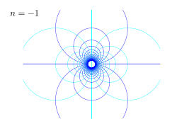
Power laws with n = −1: doublet

If $n=\,-1$, the streamlines are given by

$\psi=-\frac{A}{r}\sin\theta.$

This is more easily interpreted in terms of real and imaginary components:

$\psi = {-A y \over r^2} = {-A y \over x^2 + y^2},$

$x^2 + y^2 + {A y \over \psi} = 0,$

$x^2+\left(y+\frac{A}{2\psi}\right)^2=\left(\frac{A}{2\psi}\right)^2.$

Thus the streamlines are circles that are tangent to the x-axis at the origin. The circles in the upper half-plane thus flow clockwise, those in the lower half-plane flow anticlockwise. Note that the velocity components are proportional to r ^{− 2}; and their values at the origin is infinite. This flow pattern is usually referred to as a doublet and can be interpreted as the combination of source-sink pair of infinite strength kept at an infinitesimally small distance apart.

The velocity field is given by

$(u,v)=\left( {\partial \psi \over \partial y}, - {\partial \psi \over \partial x} \right) = \left(A\frac{y^2-x^2}{(x^2+y^2)^2},-A\frac{2xy}{(x^2+y^2)^2}\right).$

or in polar coordinates:

$(u_r, u_\theta)=\left( \frac{1}{r} {\partial \psi \over \partial \theta}, - {\partial \psi \over \partial r} \right) = \left(-\frac{A}{r^2}\cos\theta, -\frac{A}{r^2}\sin\theta\right).$

Power laws with n = −2: quadrupole

If $n=\,-2$, the streamlines are given by

$\psi=-\frac{A}{r^2}\sin(2 \theta).$

This is the flow field associated with a quadrupole.^{[citation needed]}

See also

• Stream function
• Laplacian field
• Conformal mapping
• Flownet
• Velocity potential
• Aerodynamic Potential Flow Codes

Notes

1. ^ ^{a b c d e} Batchelor (1973) pp. 99–101.
2. ^ ^{a b c} Batchelor (1973) pp. 378–380.
3. ^ Kirby, B.J. (2010), Micro- and Nanoscale Fluid Mechanics: Transport in Microfluidic Devices., Cambridge University Press, ISBN 978-0521119030, http://www.kirbyresearch.com/textbook 
4. ^ ^{a b c d} Anderson, J.D. (2002), Modern compressible flow, McGraw-Hill, ISBN 0072424435 , pp. 358–359.
5. ^ Lamb (1994) §6–§7, pp. 3–6.
6. ^ Batchelor (1973) p. 161.
7. ^ Lamb (1994) §287, pp. 492–495.
8. ^ Feynman, R.P.; Leighton, R.B.; Sands, M. (1964), The Feynman Lectures on Physics, 2, Addison-Wesley , p. 40-3. Chapter 40 has the title: The flow of dry water.
9. ^ Batchelor (1973) pp. 404–405.
10. ^ ^{a b c d e f g h i} Batchelor (1973) pp. 106–108.
11. ^ ^{a b c} Batchelor (1973) pp. 409–413.

References

• Batchelor, G.K. (1973), An introduction to fluid dynamics, Cambridge University Press, ISBN 0-521-09817-3 
• Chanson, H. (2009), Applied Hydrodynamics: An Introduction to Ideal and Real Fluid Flows, CRC Press, Taylor & Francis Group, Leiden, The Netherlands, 478 pages, ISBN 978-0-415-49271-3, http://espace.library.uq.edu.au/view/UQ:191112 

• Lamb, H. (1994) [1932], Hydrodynamics (6th ed.), Cambridge University Press, ISBN 9780521458689 
• Milne-Thomson, L.M. (1996) [1968], Theoretical hydrodynamics (5th ed.), Dover, ISBN 0486689700 

Further reading

• Chanson, H. (2007), "Le potentiel de vitesse pour les écoulements de fluides réels: la contribution de Joseph-Louis Lagrange [Velocity potential in real fluid flows: Joseph-Louis Lagrange's contribution]", La Houille Blanche (5): 127–131, doi:10.1051/lhb:2007072, http://espace.library.uq.edu.au/view/UQ:119883  (French)
• Wehausen, J.V.; Laitone, E.V. (1960), "Surface waves", in Flügge, S.; Truesdell, C., Encyclopedia of Physics, IX, Springer Verlag, pp. 446–778, http://www.coe.berkeley.edu/SurfaceWaves 

External links

• "Irrotational flow of an inviscid fluid". University of Genoa, Faculty of Engineering. http://www.diam.unige.it/~irro/lecture_e.html. Retrieved 2009-03-29. 
• "Conformal Maps Gallery". 3D-XplorMath. http://3d-xplormath.org/j/applets/en/index.html. Retrieved 2009-03-29.  — Java applets for exploring conformal maps