Boundary layer

For the anatomical structure, see Boundary layer of uterus.

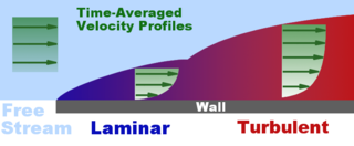Boundary layer visualization, showing transition from laminar to turbulent condition

In physics and fluid mechanics, a boundary layer is that layer of fluid in the immediate vicinity of a bounding surface where effects of viscosity of the fluid are considered in detail. In the Earth's atmosphere, the planetary boundary layer is the air layer near the ground affected by diurnal heat, moisture or momentum transfer to or from the surface. On an aircraft wing the boundary layer is the part of the flow close to the wing. The boundary layer effect occurs at the field region in which all changes occur in the flow pattern. The boundary layer distorts surrounding non-viscous flow. It is a phenomenon of viscous forces. This effect is related to the Reynolds number.

Laminar boundary layers come in various forms and can be loosely classified according to their structure and the circumstances under which they are created. The thin shear layer which develops on an oscillating body is an example of a Stokes boundary layer, while the Blasius boundary layer refers to the well-known similarity solution for the steady boundary layer attached to a flat plate held in an oncoming unidirectional flow. When a fluid rotates, viscous forces may be balanced by the Coriolis effect, rather than convective inertia, leading to the formation of an Ekman layer. Thermal boundary layers also exist in heat transfer. Multiple types of boundary layers can coexist near a surface simultaneously.

Aerodynamics

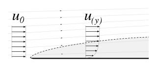Laminar boundary layer velocity profile

The aerodynamic boundary layer was first defined by Ludwig Prandtl in a paper presented on August 12, 1904 at the third International Congress of Mathematicians in Heidelberg, Germany. It allows aerodynamicists to simplify the equations of fluid flow by dividing the flow field into two areas: one inside the boundary layer, where viscosity is dominant and the majority of the drag experienced by a body immersed in a fluid is created, and one outside the boundary layer where viscosity can be neglected without significant effects on the solution. This allows a closed-form solution for the flow in both areas, which is a significant simplification over the solution of the full Navier–Stokes equations. The majority of the heat transfer to and from a body also takes place within the boundary layer, again allowing the equations to be simplified in the flow field outside the boundary layer.

The thickness of the velocity boundary layer is normally defined as the distance from the solid body at which the flow velocity is 99% of the freestream velocity, that is, the velocity that is calculated at the surface of the body in an inviscid flow solution. An alternative definition, the displacement thickness, recognises the fact that the boundary layer represents a deficit in mass flow compared to an inviscid case with slip at the wall. It is the distance by which the wall would have to be displaced in the inviscid case to give the same total mass flow as the viscous case. The no-slip condition requires the flow velocity at the surface of a solid object be zero and the fluid temperature be equal to the temperature of the surface. The flow velocity will then increase rapidly within the boundary layer, governed by the boundary layer equations, below. The thermal boundary layer thickness is similarly the distance from the body at which the temperature is 99% of the temperature found from an inviscid solution. The ratio of the two thicknesses is governed by the Prandtl number. If the Prandtl number is 1, the two boundary layers are the same thickness. If the Prandtl number is greater than 1, the thermal boundary layer is thinner than the velocity boundary layer. If the Prandtl number is less than 1, which is the case for air at standard conditions, the thermal boundary layer is thicker than the velocity boundary layer.

In high-performance designs, such as gliders and commercial transport aircraft, much attention is paid to controlling the behavior of the boundary layer to minimize drag. Two effects have to be considered. First, the boundary layer adds to the effective thickness of the body, through the displacement thickness, hence increasing the pressure drag. Secondly, the shear forces at the surface of the wing create skin friction drag.

At high Reynolds numbers, typical of full-sized aircraft, it is desirable to have a laminar boundary layer. This results in a lower skin friction due to the characteristic velocity profile of laminar flow. However, the boundary layer inevitably thickens and becomes less stable as the flow develops along the body, and eventually becomes turbulent, the process known as boundary layer transition. One way of dealing with this problem is to suck the boundary layer away through a porous surface (see Boundary layer suction). This can result in a reduction in drag, but is usually impractical due to the mechanical complexity involved and the power required to move the air and dispose of it. Natural laminar flow is the name for techniques pushing the boundary layer transition aft by shaping of an aerofoil or a fuselage so that their thickest point is aft and less thick. This reduces the velocities in the leading part and the same Reynolds number is achieved with a greater length.

At lower Reynolds numbers, such as those seen with model aircraft, it is relatively easy to maintain laminar flow. This gives low skin friction, which is desirable. However, the same velocity profile which gives the laminar boundary layer its low skin friction also causes it to be badly affected by adverse pressure gradients. As the pressure begins to recover over the rear part of the wing chord, a laminar boundary layer will tend to separate from the surface. Such flow separation causes a large increase in the pressure drag, since it greatly increases the effective size of the wing section. In these cases, it can be advantageous to deliberately trip the boundary layer into turbulence at a point prior to the location of laminar separation, using a turbulator. The fuller velocity profile of the turbulent boundary layer allows it to sustain the adverse pressure gradient without separating. Thus, although the skin friction is increased, overall drag is decreased. This is the principle behind the dimpling on golf balls, as well as vortex generators on aircraft. Special wing sections have also been designed which tailor the pressure recovery so laminar separation is reduced or even eliminated. This represents an optimum compromise between the pressure drag from flow separation and skin friction from induced turbulence.

Naval architecture

Many of the principles that apply to aircraft also apply to ships, submarines, and offshore platforms.

For ships, unlike aircraft, the principle behind fluid dynamics would be incompressible flows (because the change in density of water when the pressure rises close to 1000kPa would be only 2–3 kg m⁻³). The field of fluid dynamics that deals with incompressible fluids is called hydrodynamics. From an engineer's point of view, for a ship, the basic design would be a design for hydrodynamics, and later followed by a design for strength. The boundary layer development, break down and separation becomes very critical, as the shear stresses experienced by the parts would be high due to the high viscosity of water. Also, the slip stream effect (assume the ship to be a spear tearing through sponge at very high velocity) becomes very prominent, due to the high viscosity.

Boundary layer equations

The deduction of the boundary layer equations was perhaps one of the most important advances in fluid dynamics. Using an order of magnitude analysis, the well-known governing Navier–Stokes equations of viscous fluid flow can be greatly simplified within the boundary layer. Notably, the characteristic of the partial differential equations (PDE) becomes parabolic, rather than the elliptical form of the full Navier–Stokes equations. This greatly simplifies the solution of the equations. By making the boundary layer approximation, the flow is divided into an inviscid portion (which is easy to solve by a number of methods) and the boundary layer, which is governed by an easier to solve PDE. The continuity and Navier–Stokes equations for a two-dimensional steady incompressible flow in Cartesian coordinates are given by

${\partial u\over\partial x}+{\partial \upsilon\over\partial y}=0$

$u{\partial u \over \partial x}+\upsilon{\partial u \over \partial y}=-{1\over \rho} {\partial p \over \partial x}+{\nu}\left({\partial^2 u\over \partial x^2}+{\partial^2 u\over \partial y^2}\right)$

$u{\partial \upsilon \over \partial x}+\upsilon{\partial \upsilon \over \partial y}=-{1\over \rho} {\partial p \over \partial y}+{\nu}\left({\partial^2 \upsilon\over \partial x^2}+{\partial^2 \upsilon\over \partial y^2}\right)$

where u and υ are the velocity components, ρ is the density, p is the pressure, and ν is the kinematic viscosity of the fluid at a point.

The approximation states that, for a sufficiently high Reynolds number the flow over a surface can be divided into an outer region of inviscid flow unaffected by viscosity (the majority of the flow), and a region close to the surface where viscosity is important (the boundary layer). Let u and υ be streamwise and transverse (wall normal) velocities respectively inside the boundary layer. Using scale analysis, it can be shown that the above equations of motion reduce within the boundary layer to become

${\partial u\over\partial x}+{\partial \upsilon\over\partial y}=0$

$u{\partial u \over \partial x}+\upsilon{\partial u \over \partial y}=-{1\over \rho} {\partial p \over \partial x}+{\nu}{\partial^2 u\over \partial y^2}$

and if the fluid is incompressible (as liquids are under standard conditions):

${1\over \rho} {\partial p \over \partial y}=0$

The asymptotic analysis also shows that υ, the wall normal velocity, is small compared with u the streamwise velocity, and that variations in properties in the streamwise direction are generally much lower than those in the wall normal direction.

Since the static pressure p is independent of y, then pressure at the edge of the boundary layer is the pressure throughout the boundary layer at a given streamwise position. The external pressure may be obtained through an application of Bernoulli's equation. Let u₀ be the fluid velocity outside the boundary layer, where u and u₀ are both parallel. This gives upon substituting for p the following result

$u{\partial u \over \partial x}+\upsilon{\partial u \over \partial y}=u_0{\partial u_0 \over \partial x}+{\nu}{\partial^2 u\over \partial y^2}$

with the boundary condition

${\partial u\over\partial x}+{\partial v\over\partial y}=0$

For a flow in which the static pressure p also does not change in the direction of the flow then

${\partial p\over\partial x}=0$

so u₀ remains constant.

Therefore, the equation of motion simplifies to become

$u{\partial u \over \partial x}+\upsilon{\partial u \over \partial y}={\nu}{\partial^2 u\over \partial y^2}$

These approximations are used in a variety of practical flow problems of scientific and engineering interest. The above analysis is for any instantaneous laminar or turbulent boundary layer, but is used mainly in laminar flow studies since the mean flow is also the instantaneous flow because there are no velocity fluctuations present.

Turbulent boundary layers

The treatment of turbulent boundary layers is far more difficult due to the time-dependent variation of the flow properties. One of the most widely used techniques in which turbulent flows are tackled is to apply Reynolds decomposition. Here the instantaneous flow properties are decomposed into a mean and fluctuating component. Applying this technique to the boundary layer equations gives the full turbulent boundary layer equations not often given in literature:

${\partial \overline{u}\over\partial x}+{\partial \overline{v}\over\partial y}=0$

$\overline{u}{\partial \overline{u} \over \partial x}+\overline{v}{\partial \overline{u} \over \partial y}=-{1\over \rho} {\partial \overline{p} \over \partial x}+ \nu \left({\partial^2 \overline{u}\over \partial x^2}+{\partial^2 \overline{u}\over \partial y^2}\right)-\frac{\partial}{\partial y}(\overline{u'v'})-\frac{\partial}{\partial x}(\overline{u'^2})$

$\overline{u}{\partial \overline{v} \over \partial x}+\overline{v}{\partial \overline{v} \over \partial y}=-{1\over \rho} {\partial \overline{p} \over \partial y}+\nu \left({\partial^2 \overline{v}\over \partial x^2}+{\partial^2 \overline{v}\over \partial y^2}\right)-\frac{\partial}{\partial x}(\overline{u'v'})-\frac{\partial}{\partial y}(\overline{v'^2})$

Using the same order-of-magnitude analysis as for the instantaneous equations, these turbulent boundary layer equations generally reduce to become in their classical form:

${\partial \overline{u}\over\partial x}+{\partial \overline{v}\over\partial y}=0$

$\overline{u}{\partial \overline{u} \over \partial x}+\overline{v}{\partial \overline{u} \over \partial y}=-{1\over \rho} {\partial \overline{p} \over \partial x}+{\nu}{\partial^2 \overline{u}\over \partial y^2}-\frac{\partial}{\partial y}(\overline{u'v'})$

${\partial \overline{p} \over \partial y}=0$

The additional term $\overline{u'v'}$ in the turbulent boundary layer equations is known as the Reynolds shear stress and is unknown a priori. The solution of the turbulent boundary layer equations therefore necessitates the use of a turbulence model, which aims to express the Reynolds shear stress in terms of known flow variables or derivatives. The lack of accuracy and generality of such models is a major obstacle in the successful prediction of turbulent flow properties in modern fluid dynamics.

Boundary layer turbine

This effect was exploited in the Tesla turbine, patented by Nikola Tesla in 1913. It is referred to as a bladeless turbine because it uses the boundary layer effect and not a fluid impinging upon the blades as in a conventional turbine. Boundary layer turbines are also known as cohesion-type turbine, bladeless turbine, and Prandtl layer turbine (after Ludwig Prandtl).

See also

• Boundary layer separation
• Boundary-layer thickness
• Boundary layer suction
• Boundary layer control
• Coandă effect
• Facility for Airborne Atmospheric Measurements
• Logarithmic law of the wall
• Planetary boundary layer
• Shape factor (boundary layer flow)
• Shear stress

References

• Chanson, H. (2009). Applied Hydrodynamics: An Introduction to Ideal and Real Fluid Flows. CRC Press, Taylor & Francis Group, Leiden, The Netherlands, 478 pages. ISBN 978-0-415-49271-3. http://espace.library.uq.edu.au/view/UQ:191112. 
• A.D. Polyanin and V.F. Zaitsev, Handbook of Nonlinear Partial Differential Equations, Chapman & Hall/CRC Press, Boca Raton - London, 2004. ISBN 1-58488-355-3
• A.D. Polyanin, A.M. Kutepov, A.V. Vyazmin, and D.A. Kazenin, Hydrodynamics, Mass and Heat Transfer in Chemical Engineering, Taylor & Francis, London, 2002. ISBN 0-415-27237-8
• Hermann Schlichting, Klaus Gersten, E. Krause, H. Jr. Oertel, C. Mayes "Boundary-Layer Theory" 8th edition Springer 2004 ISBN 3-540-66270-7
• John D. Anderson, Jr., "Ludwig Prandtl's Boundary Layer", Physics Today, December 2005
• Anderson, John (1992). Fundamentals of Aerodynamics (2nd edition ed.). Toronto: S.S.CHAND. pp. 711–714. ISBN 0-07-001679-8. 
• H. Tennekes and J. L. Lumley, "A First Course in Turbulence", The MIT Press, (1972).

External links

• National Science Digital Library - Boundary Layer
• Moore, Franklin K., "Displacement effect of a three-dimensional boundary layer". NACA Report 1124, 1953.
• Benson, Tom, "Boundary layer". NASA Glenn Learning Technologies.
• Boundary layer separation
• Boundary layer equations: Exact Solutions - from EqWorld