Differential of a function

For other uses of differential in mathematics, see differential (mathematics).

In calculus, the differential represents the principal part of the change in a function y = ƒ(x) with respect to changes in the independent variable. The differential dy is defined by

$dy = f'(x)\,dx,$

where f'(x) is the derivative of ƒ with respect to x, and dx is an additional real variable (so that dy is a function of x and dx). The notation is such that the equation

$dy = \frac{dy}{dx}\, dx$

holds, where the derivative is represented in the Leibniz notation dy/dx, and this is consistent with regarding the derivative as the quotient of the differentials. One also writes

$df(x) = f'(x)\,dx.$

The precise meaning of the variables dy and dx depends on the context of the application and the required level of mathematical rigor. The domain of these variables may take on a particular geometrical significance if the differential is regarded as a particular differential form, or analytical significance if the differential is regarded as a linear approximation to the increment of a function. In physical applications, the variables dx and dy are often constrained to be very small ("infinitesimal").

History and usage

The differential was first introduced via an intuitive or heuristic definition by Gottfried Wilhelm Leibniz, who thought of the differential dy as an infinitely small (or infinitesimal) change in the value y of the function, corresponding to an infinitely small change dx in the function's argument x. For that reason, the instantaneous rate of change of y with respect to x, which is the value of the derivative of the function, is denoted by the fraction

$\frac{dy}{dx}$

in what is called the Leibniz notation for derivatives. The quotient dy/dx is not infinitely small; rather it is a real number.

The use of infinitesimals in this form was widely criticized, for instance by the famous pamphlet The Analyst by Bishop Berkeley. Augustin-Louis Cauchy (1823) defined the differential without appeal to the atomism of Leibniz's infinitesimals.^[1][2] Instead, Cauchy, following d'Alembert, inverted the logical order of Leibniz and his successors: the derivative itself became the fundamental object, defined as a limit of difference quotients, and the differentials were then defined in terms of it. That is, one was free to define the differential dy by an expression

$dy = f'(x)\,dx$

in which dy and dx are simply new variables taking finite real values,^[3] not fixed infinitesimals as they had been for Leibniz.^[4]

According to Boyer (1959, p. 12), Cauchy's approach was a significant logical improvement over the infinitesimal approach of Leibniz because, instead of invoking the metaphysical notion of infinitesimals, the quantities dy and dx could now be manipulated in exactly the same manner as any other real quantities in a meaningful way. Cauchy's overall conceptual approach to differentials remains the standard one in modern analytical treatments,^[5] although the final word on rigor, a fully modern notion of the limit, was ultimately due to Karl Weierstrass.^[6]

In physical treatments, such as those applied to the theory of thermodynamics, the infinitesimal view still prevails. Courant & John (1999, p. 184) reconcile the physical use of infinitesimal differentials with the mathematical impossibility of them as follows. The differentials represent finite non-zero values that are smaller than the degree of accuracy required for the particular purpose for which they are intended. Thus "physical infinitesimals" need not appeal to a corresponding mathematical infinitesimal in order to have a precise sense.

Following twentieth-century developments in mathematical analysis and differential geometry, it became clear that the notion of the differential of a function could be extended in a variety of ways. In real analysis, it is more desirable to deal directly with the differential as the principal part of the increment of a function. This leads directly to the notion that the differential of a function at a point is linear functional of an increment Δx. This approach allows the differential (as a linear map) to be developed for a variety of more sophisticated spaces, ultimately giving rise to such notions as the Fréchet or Gâteaux derivative. Likewise, in differential geometry, the differential of a function at a point is a linear function of a tangent vector (an "infinitely small displacement"), which exhibits it as a kind of one-form: the exterior derivative of the function. In non-standard calculus, differentials are regarded as infinitesimals, which can themselves be put on a rigorous footing (see differential (infinitesimal)).

Definition

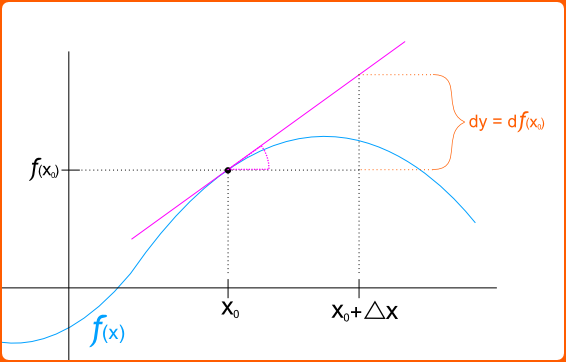
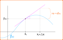The differential of a function ƒ(x) at a point x₀.

The differential is defined in modern treatments of differential calculus as follows.^[7] The differential of a function ƒ(x) of a single real variable x is the function df of two independent real variables x and Δx given by

$df(x, \Delta x) \stackrel{\rm{def}}{=} f'(x)\,\Delta x.$

One or both of the arguments may be suppressed, i.e., one may see df(x) or simply df. If y = ƒ(x), the differential may also be written as dy. Since dx(x, Δx) = Δx it is conventional to write dx = Δx, so that the following equality holds:

$df(x) = f'(x) \, dx$

This notion of differential is broadly applicable when a linear approximation to a function is sought, in which the value of the increment Δx is small enough. More precisely, if ƒ is a differentiable function at x, then the difference in y-values

$\Delta y \stackrel{\rm{def}}{=} f(x+\Delta x) - f(x)$

satisfies

$\Delta y = f'(x)\,\Delta x + \varepsilon = df(x) + \varepsilon\,$

where the error ε in the approximation satisfies ε/Δx → 0 as Δx → 0. In other words, one has the approximate identity

$\Delta y \approx dy$

in which the error can be made as small as desired relative to Δx by constraining Δx to be sufficiently small; that is to say,

$\frac{\Delta y - dy}{\Delta x}\to 0$

as Δx → 0. For this reason, the differential of a function is known as the principal (linear) part in the increment of a function: the differential is a linear function of the increment Δx, and although the error ε may be nonlinear, it tends to zero rapidly as Δx tends to zero.

Differentials in several variables

Following Goursat (1904, I, §15), for functions of more than one independent variable,

$y = f(x_1,\dots,x_n), \,$

the partial differential of y with respect to any one of the variables x₁ is the principal part of the change in y resulting from a change dx₁ in that one variable. The partial differential is therefore

$\frac{\partial y}{\partial x_1} dx_1$

involving the partial derivative of y with respect to x₁. The sum of the partial differentials with respect to all of the independent variables is the total differential

$dy = \frac{\partial y}{\partial x_1} dx_1 + \cdots + \frac{\partial y}{\partial x_n} dx_n,$

which is the principal part of the change in y resulting from changes in the independent variables x _i.

More precisely, in the context of multivariable calculus, following Courant (1937ii), if ƒ is a differentiable function, then by the definition of the differentiability, the increment

$\begin{align} \Delta y &{}\stackrel{\mathrm{def}}{=} f(x_1+\Delta x_1, \dots, x_n+\Delta x_n) - f(x_1,\dots,x_n)\\ &{}= \frac{\partial y}{\partial x_1} \Delta x_1 + \cdots + \frac{\partial y}{\partial x_n} \Delta x_n + \varepsilon_1\Delta x_1 +\cdots+\varepsilon_n\Delta x_n \end{align}$

where the error terms ε _i tend to zero as the increments Δx_i jointly tend to zero. The total differential is then rigorously defined as

$dy = \frac{\partial y}{\partial x_1} \Delta x_1 + \cdots + \frac{\partial y}{\partial x_n} \Delta x_n.$

Since, with this definition,

$dx_i(\Delta x_1,\dots,\Delta x_n) = \Delta x_i,$

one has

$dy = \frac{\partial y}{\partial x_1}\,d x_1 + \cdots + \frac{\partial y}{\partial x_n}\,d x_n.$

As in the case of one variable, the approximate identity holds

$dy \approx \Delta y$

in which the total error can be made as small as desired relative to $\sqrt{\Delta x_1^2+\cdots +\Delta x_n^2}$ by confining attention to sufficiently small increments.

Higher-order differentials

Higher-order differentials of a function y = ƒ(x) of a single variable x can be defined via:^[8]

$d^2y = d(dy) = d(f'(x)dx) = f''(x)\,(dx)^2,$

and, in general,

$d^ny = f^{(n)}(x)\,(dx)^n.$

Informally, this justifies Leibniz's notation for higher-order derivatives

$f^{(n)}(x) = \frac{d^n f}{dx^n}.$

When the independent variable x itself is permitted to depend on other variables, then the expression becomes more complicated, as it must include also higher order differentials in x itself. Thus, for instance,

$\begin{align} d^2 y &= f''(x)\,(dx)^2 + f'(x)d^2x\\ d^3 y &= f'''(x)\, (dx)^3 + 3f''(x)dx\,d^2x + f'(x)d^3x \end{align}$

and so forth.

Similar considerations apply to defining higher order differentials of functions of several variables. For example, if ƒ is a function of two variables x and y, then

$d^nf = \sum_{k=0}^n \binom{n}{k}\frac{\partial^kf}{\partial x^k}\frac{\partial^{n-k}f}{\partial y^{n-k}}(dx)^k(dy)^{n-k},$

where $\scriptstyle{\binom{n}{k}}$ is a binomial coefficient. In more variables, an analogous expression holds, but with an appropriate multinomial expansion rather than binomial expansion.^[9]

Higher order differentials in several variables also become more complicated when the independent variables are themselves allowed to depend on other variables. For instance, for a function ƒ of x and y which are allowed to depend on auxiliary variables, one has

$d^2f = \left(\frac{\partial^2f}{\partial x^2}(dx)^2+2\frac{\partial^2f}{\partial x\partial y}dx\,dy + \frac{\partial^2f}{\partial y^2}(dy)^2\right) + \frac{\partial f}{\partial x}d^2x + \frac{\partial f}{\partial y}d^2y.$

Because of this notational infelicity, the use of higher order differentials was roundly criticized by Hadamard 1935, who concluded:

Enfin, que signifie ou que représente l'égalité

$d^2z = r\,dx^2 + 2s\,dx\,dy + t\,dy^2\,?$

A mon avis, rien du tout.

That is: Finally, what is meant, or represented, by the equality [...]? In my opinion, nothing at all. In spite of this skepticism, higher order differentials did emerge as an important tool in analysis^[10]

In these contexts, the nth order differential of the function ƒ applied to an increment Δx is defined by

$d^nf(x,\Delta x) = \left.\frac{d^n}{dt^n} f(x+t\Delta x)\right|_{t=0}$

or an equivalent expression, such as

$\lim_{t\to 0}\frac{\Delta^n_{t\Delta x} f}{t^n}$

where $\Delta^n_{t\Delta x} f$ is an nth forward difference with increment tΔx.

This definition makes sense as well if ƒ is a function of several variables (for simplicity taken here as a vector argument). Then the nth differential defined in this way is a homogeneous function of degree n in the vector increment Δx. Furthermore, the Taylor series of ƒ at the point x is given by

$f(x+\Delta x)\sim f(x) + df(x,\Delta x) + \frac{1}{2}d^2f(x,\Delta x) + \cdots + \frac{1}{n!}d^nf(x,\Delta x) + \cdots$

The higher order Gâteaux derivative generalizes these considerations to infinite dimensional spaces.

Properties

A number of properties of the differential follow in a straightforward manner from the corresponding properties of the derivative, partial derivative, and total derivative. These include:^[11]

• Linearity: For constants a and b and differentiable functions ƒ and g,

$d(af+bg) = a\,df + b\,dg.$

• Product rule: For two differentiable functions ƒ and g,

$d(fg) = f\,dg+g\,df.$

An operation d with these two properties is known in abstract algebra as a derivation. In addition, various forms of the chain rule hold, in increasing level of generality:^[12]

• If y = ƒ(u) is a differentiable function of the variable u and u = g(x) is a differentiable function of x, then

$dy = f'(u)\,du = f'(g(x))g'(x)\,dx.$

• If y = ƒ(x₁, ..., x_n) and all of the variables x₁, ..., x_n depend on another variable t, then by the chain rule for partial derivatives, one has

$\begin{align} dy &= \frac{dy}{dt}dt \\ &= \frac{\partial y}{\partial x_1} dx_1 + \cdots + \frac{\partial y}{\partial x_n} dx_n\\ &= \frac{\partial y}{\partial x_1} \frac{dx_1}{dt}\,dt + \cdots + \frac{\partial y}{\partial x_n} \frac{dx_n}{dt}\,dt. \end{align}$

Heuristically, the chain rule for several variables can itself be understood by dividing through both sides of this equation by the infinitely small quantity dt.

• More general analogous expressions hold, in which the intermediate variables x _i depend on more than one variable.

General formulation

See also: Fréchet derivative and Gâteaux derivative

A consistent notion of differential can be developed for a function ƒ Rⁿ → R^m between two Euclidean spaces. Let x,Δx ∈ Rⁿ be a pair of Euclidean vectors. The increment in the function ƒ is

$\Delta f = f(\mathbf{x}+\Delta\mathbf{x}) - f(\mathbf{x}).$

If there exists an m × n matrix A such that

$\Delta f = A\Delta\mathbf{x} + \|\Delta\mathbf{x}\|\boldsymbol{\varepsilon}$

in which the vector ε → 0 as Δx → 0, then ƒ is by definition differentiable at the point x. The matrix A is sometimes known as the Jacobian matrix, and the linear transformation that associates to the increment Δx ∈ Rⁿ the vector AΔx ∈ R^m is, in this general setting, known as the differential dƒ(x) of ƒ at the point x. This is precisely the Fréchet derivative, and the same construction can be made to work for a function between any Banach spaces.

Another fruitful point of view is to define the differential directly as a kind of directional derivative:

$df(\mathbf{x},\mathbf{h}) = \lim_{t\to 0}\frac{f(\mathbf{x}+t\mathbf{h})-f(\mathbf{x})}{t} = \left.\frac{d}{dt}f(\mathbf{x}+t\mathbf{h})\right|_{t=0},$

which is the approach already taken for defining higher order differentials (and is most nearly the definition set forth by Cauchy). If t represents time and x position, then h represents a velocity instead of a displacement as we have heretofore regarded it. This yields yet another refinement of the notion of differential: that it should be a linear function of a kinematic velocity. The set of all velocities through a given point of space is known as the tangent space, and so dƒ gives a linear function on the tangent space: a differential form. With this interpretation, the differential of ƒ is known as the exterior derivative, and has broad application in differential geometry because the notion of velocities and the tangent space makes sense on any differentiable manifold. If, in addition, the output value of ƒ also represents a position (in a Euclidean space), then a dimensional analysis confirms that the output value of dƒ must be a velocity. If one treats the differential in this manner, then it is known as the pushforward since it "pushes" velocities from a source space into velocities in a target space.

Other approaches

Main article: Differential (infinitesimal)

Although the notion of having an infinitesimal increment dx is not well-defined in modern mathematical analysis, a variety of techniques exist for defining the infinitesimal differential so that the differential of a function can be handled in a manner that does not clash with the Leibniz notation. These include:

• Defining the differential as a kind of differential form, specifically the exterior derivative of a function. The infinitesimal increments are then identified with vectors in the tangent space at a point. This approach is popular in differential geometry and related fields, because it readily generalizes to mappings between differentiable manifolds.
• Differentials as nilpotent elements of commutative rings. This approach is popular in algebraic geometry.^[13]
• Differentials in smooth models of set theory. This approach is known as synthetic differential geometry or smooth infinitesimal analysis and is closely related to the algebraic geometric approach, except that ideas from topos theory are used to hide the mechanisms by which nilpotent infinitesimals are introduced.^[14]
• Differentials as infinitesimals in hyperreal number systems, which are extensions of the real numbers which contain invertible infinitesimals and infinitely large numbers. This is the approach of nonstandard analysis pioneered by Abraham Robinson.^[15]

Examples and applications

Differentials may be effectively used in numerical analysis to study the propagation of experimental errors in a calculation, and thus the overall numerical stability of a problem (Courant 1937i). Suppose that the variable x represents the outcome of an experiment and y is the result of a numerical computation applied to x. The question is to what extent errors in the measurement of x influence the outcome of the computation of y. If the x is known to within Δx of its true value, then Taylor's theorem gives the following estimate on the error Δy in the computation of y:

$\Delta y = f'(x)\Delta x + \frac{(\Delta x)^2}{2}f''(\xi)$

where ξ = x + θΔx for some 0 < θ < 1. If Δx is small, then the second order term is negligible, so that Δy is, for practical purposes, well-approximated by dy = ƒ'(x)Δx.

The differential is often useful to rewrite a differential equation

$\frac{dy}{dx} = g(x)$

in the form

$dy = g(x)\,dx,$

in particular when one wants to separate the variables.

Notes

1. ^ For a detailed historical account of the differential, see Boyer 1959, especially page 275 for Cauchy's contribution on the subject. An abbreviated account appears in Kline 1972, Chapter 40.
2. ^ Cauchy explicitly denied the possibility of actual infinitesimal and infinite quantities (Boyer 1959, pp. 273–275), and took the radically different point of view that "a variable quantity becomes infinitely small when its numerical value decreases indefinitely in such a way as to converge to zero" (Cauchy 1823, p. 12; translation from Boyer 1959, p. 273).
3. ^ Boyer 1959, p. 275
4. ^ Boyer 1959, p. 12: "The differentials as thus defined are only new variables, and not fixed infinitesimals..."
5. ^ Courant 1937i, II, §9: "Here we remark merely in passing that it is possible to use this approximate representation of the increment Δy by the linear expression hƒ(x) to construct a logically satisfactory definition of a "differential", as was done by Cauchy in particular."
6. ^ Boyer 1959, p. 284
7. ^ See, for instance, the influential treatises of Courant 1937i, Kline 1977, Goursat 1904, and Hardy 1905. Tertiary sources for this definition include also Tolstov 2001 and Ito 1993, §106.
8. ^ Cauchy 1823. See also, for instance, Goursat 1904, I, §14.
9. ^ Goursat 1904, I, §14
10. ^ In particular to infinite dimensional holomorphy (Hille & Phillips 1974) and numerical analysis via the calculus of finite differences.
11. ^ Goursat 1904, I, §17
12. ^ Goursat 1904, I, §§14,16
13. ^ Eisenbud & Harris 1998.
14. ^ See Kock 2006 and Moerdijk & Reyes 1991.
15. ^ See Robinson 1996 and Keisler 1986.

References

• Boyer, Carl B. (1959), The history of the calculus and its conceptual development, New York: Dover Publications, MR0124178 .
• Cauchy, Augustin-Louis (1823), Résumé des Leçons données à l'Ecole royale polytechnique sur les applications du calcul infinitésimal, http://math-doc.ujf-grenoble.fr/cgi-bin/oeitem?id=OE_CAUCHY_2_4_9_0 .
• Courant, Richard (1937i), Differential and integral calculus. Vol. I, Wiley Classics Library, New York: John Wiley & Sons (published 1988), ISBN 978-0-471-60842-4, MR1009558 .
• Courant, Richard (1937ii), Differential and integral calculus. Vol. II, Wiley Classics Library, New York: John Wiley & Sons (published 1988), ISBN 978-0-471-60840-0, MR1009559 .
• Courant, Richard; John, Fritz (1999), Introduction to Calculus and Analysis Volume 1, Classics in Mathematics, Berlin, New York: Springer-Verlag, ISBN 3-540-65058-X, MR1746554 
• Eisenbud, David; Harris, Joe (1998), The Geometry of Schemes, Springer-Verlag, ISBN 0-387-98637-5 .
• Fréchet, Maurice (1925), "La notion de différentielle dans l'analyse générale", Annales Scientifiques de l'École Normale Supérieure. Troisième Série 42: 293–323, ISSN 0012-9593, MR1509268 .
• Goursat, Édouard (1904), A course in mathematical analysis: Vol 1: Derivatives and differentials, definite integrals, expansion in series, applications to geometry, E. R. Hedrick, New York: Dover Publications (published 1959), MR0106155, http://www.archive.org/details/coursemathanalys01gourrich .
• Hadamard, Jacques (1935), "La notion de différentiel dans l'enseignement", Mathematical Gazette XIX (236): 341–342, JSTOR 3606323 .
• Hardy, Godfrey Harold (1908), A Course of Pure Mathematics, Cambridge University Press, ISBN 978-0-521-09227-2 .
• Hille, Einar; Phillips, Ralph S. (1974), Functional analysis and semi-groups, Providence, R.I.: American Mathematical Society, MR0423094 .
• Ito, Kiyosi (1993), Encyclopedic Dictionary of Mathematics (2nd ed.), MIT Press, ISBN 978-0-262-59020-4 .
• Kline, Morris (1977), "Chapter 13: Differentials and the law of the mean", Calculus: An intuitive and physical approach, John Wiley and Sons .
• Kline, Morris (1972), Mathematical thought from ancient to modern times (3rd ed.), Oxford University Press (published 1990), ISBN 978-0-19-506136-9 
• Keisler, H. Jerome (1986), Elementary Calculus: An Infinitesimal Approach (2nd ed.), http://www.math.wisc.edu/~keisler/calc.html .
• Kock, Anders (2006), Synthetic Differential Geometry (2nd ed.), Cambridge University Press, http://home.imf.au.dk/kock/sdg99.pdf .
• Moerdijk, I.; Reyes, G.E. (1991), Models for Smooth Infinitesimal Analysis, Springer-Verlag .
• Robinson, Abraham (1996), Non-standard analysis, Princeton University Press, ISBN 978-0-691-04490-3 .
• Tolstov, G.P. (2001), "Differential", in Hazewinkel, Michiel, Encyclopaedia of Mathematics, Springer, ISBN 978-1556080104, http://eom.springer.de/D/d031810.htm .

External links

• Differential Of A Function at Wolfram Demonstrations Project