Taylor series

"Series expansion" redirects here. For other notions of the term, see series (mathematics).

As the degree of the Taylor polynomial rises, it approaches the correct function. This image shows sin x (in black) and Taylor approximations, polynomials of degree 1, 3, 5, 7, 9, 11 and 13.

The exponential function (in blue), and the sum of the first n+1 terms of its Taylor series at 0 (in red).

In mathematics, a Taylor series is a representation of a function as an infinite sum of terms that are calculated from the values of the function's derivatives at a single point.

The concept of a Taylor series was formally introduced by the English mathematician Brook Taylor in 1715. If the Taylor series is centered at zero, then that series is also called a Maclaurin series, named after the Scottish mathematician Colin Maclaurin, who made extensive use of this special case of Taylor series in the 18th century.

It is common practice to approximate a function by using a finite number of terms of its Taylor series. Taylor's theorem gives quantitative estimates on the error in this approximation. Any finite number of initial terms of the Taylor series of a function is called a Taylor polynomial. The Taylor series of a function is the limit of that function's Taylor polynomials, provided that the limit exists. A function may not be equal to its Taylor series, even if its Taylor series converges at every point. A function that is equal to its Taylor series in an open interval (or a disc in the complex plane) is known as an analytic function.

Definition

The Taylor series of a real or complex function ƒ(x) that is infinitely differentiable in a neighborhood of a real or complex number a is the power series

$f(a)+\frac {f'(a)}{1!} (x-a)+ \frac{f''(a)}{2!} (x-a)^2+\frac{f^{(3)}(a)}{3!}(x-a)^3+ \cdots.$

which can be written in the more compact sigma notation as

$\sum_{n=0} ^ {\infin } \frac {f^{(n)}(a)}{n!} \, (x-a)^{n}$

where n! denotes the factorial of n and ƒ ⁽ⁿ⁾(a) denotes the nth derivative of ƒ evaluated at the point a. The zeroth derivative of ƒ is defined to be ƒ itself and (x − a)⁰ and 0! are both defined to be 1. In the case that a = 0, the series is also called a Maclaurin series.

Examples

The Maclaurin series for any polynomial is the polynomial itself.

The Maclaurin series for (1 − x)⁻¹ for |x| < 1 is the geometric series

$1+x+x^2+x^3+\cdots\!$

so the Taylor series for x⁻¹ at a = 1 is

$1-(x-1)+(x-1)^2-(x-1)^3+\cdots.\!$

By integrating the above Maclaurin series we find the Maclaurin series for log(1 − x), where log denotes the natural logarithm:

$-x-\frac{1}{2}x^2-\frac{1}{3}x^3-\frac{1}{4}x^4-\cdots\!$

and the corresponding Taylor series for log(x) at a = 1 is

$(x-1)-\frac{1}{2}(x-1)^2+\frac{1}{3}(x-1)^3-\frac{1}{4}(x-1)^4+\cdots.\!$

The Taylor series for the exponential function e^x at a = 0 is

$1 + \frac{x^1}{1!} + \frac{x^2}{2!} + \frac{x^3}{3!} + \frac{x^4}{4!} + \frac{x^5}{5!}+ \cdots = 1 + x + \frac{x^2}{2} + \frac{x^3}{6} + \frac{x^4}{24} + \frac{x^5}{120} + \cdots.\!$

The above expansion holds because the derivative of e^x with respect to x is also e^x and e⁰ equals 1. This leaves the terms (x − 0)ⁿ in the numerator and n! in the denominator for each term in the infinite sum.

History

The Greek philosopher Zeno considered the problem of summing an infinite series to achieve a finite result, but rejected it as an impossibility: the result was Zeno's paradox. Later, Aristotle proposed a philosophical resolution of the paradox, but the mathematical content was apparently unresolved until taken up by Democritus and then Archimedes. It was through Archimedes's method of exhaustion that an infinite number of progressive subdivisions could be performed to achieve a finite result.^[1] Liu Hui independently employed a similar method a few centuries later.^[2]

In the 14th century, the earliest examples of the use of Taylor series and closely related methods were given by Madhava of Sangamagrama.^[3] Though no record of his work survives, writings of later Indian mathematicians suggest that he found a number of special cases of the Taylor series, including those for the trigonometric functions of sine, cosine, tangent, and arctangent. The Kerala school of astronomy and mathematics further expanded his works with various series expansions and rational approximations until the 16th century.

In the 17th century, James Gregory also worked in this area and published several Maclaurin series. It was not until 1715 however that a general method for constructing these series for all functions for which they exist was finally provided by Brook Taylor,^[4] after whom the series are now named.

The Maclaurin series was named after Colin Maclaurin, a professor in Edinburgh, who published the special case of the Taylor result in the 18th century.

Analytic functions

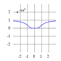The function e^−1/x² is not analytic at x = 0: the Taylor series is identically 0, although the function is not.

If f(x) is given by a convergent power series in an open disc (or interval in the real line) centered at b, it is said to be analytic in this disc. Thus for x in this disc, f is given by a convergent power series

$f(x) = \sum_{n=0}^\infty a_n(x-b)^n.$

Differentiating by x the above formula n times, then setting x=b gives:

$\frac{f^{(n)}(b)}{n!} = a_n$

and so the power series expansion agrees with the Taylor series. Thus a function is analytic in an open disc centered at b if and only if its Taylor series converges to the value of the function at each point of the disc.

If f(x) is equal to its Taylor series everywhere it is called entire. The polynomials and the exponential function e^x and the trigonometric functions sine and cosine are examples of entire functions. Examples of functions that are not entire include the logarithm, the trigonometric function tangent, and its inverse arctan. For these functions the Taylor series do not converge if x is far from a. Taylor series can be used to calculate the value of an entire function in every point, if the value of the function, and of all of its derivatives, are known at a single point.

Uses of the Taylor series for analytic functions include:

1. The partial sums (the Taylor polynomials) of the series can be used as approximations of the entire function. These approximations are good if sufficiently many terms are included.
2. Differentiation and integration of power series can be performed term by term and is hence particularly easy.
3. An analytic function is uniquely extended to a holomorphic function on an open disk in the complex plane. This makes the machinery of complex analysis available.
4. The (truncated) series can be used to compute function values numerically, (often by recasting the polynomial into the Chebyshev form and evaluating it with the Clenshaw algorithm).
5. Algebraic operations can be done readily on the power series representation; for instance the Euler's formula follows from Taylor series expansions for trigonometric and exponential functions. This result is of fundamental importance in such fields as harmonic analysis.

Approximation and convergence

The sine function (blue) is closely approximated by its Taylor polynomial of degree 7 (pink) for a full period centered at the origin.

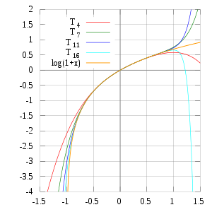The Taylor polynomials for log(1+x) only provide accurate approximations in the range −1 < x ≤ 1. Note that, for x > 1, the Taylor polynomials of higher degree are worse approximations.

Pictured on the right is an accurate approximation of sin(x) around the point x = 0. The pink curve is a polynomial of degree seven:

$\sin\left( x \right) \approx x - \frac{x^3}{3!} + \frac{x^5}{5!} - \frac{x^7}{7!}.\!$

The error in this approximation is no more than |x|⁹/9!. In particular, for −1 < x < 1, the error is less than 0.000003.

In contrast, also shown is a picture of the natural logarithm function log(1 + x) and some of its Taylor polynomials around a = 0. These approximations converge to the function only in the region −1 < x ≤ 1; outside of this region the higher-degree Taylor polynomials are worse approximations for the function. This is similar to Runge's phenomenon.

The error incurred in approximating a function by its nth-degree Taylor polynomial is called the remainder or residual and is denoted by the function R_n(x). Taylor's theorem can be used to obtain a bound on the size of the remainder.

In general, Taylor series need not be convergent at all. And in fact the set of functions with a convergent Taylor series is a meager set in the Fréchet space of smooth functions. Even if the Taylor series of a function f does converge, its limit need not in general be equal to the value of the function f(x). For example, the function

$f(x) = \begin{cases} e^{-1/x^2}&\mathrm{if}\ x\not=0\\ 0&\mathrm{if}\ x=0 \end{cases}$

is infinitely differentiable at x = 0, and has all derivatives zero there. Consequently, the Taylor series of f(x) about x = 0 is identically zero. However, f(x) is not equal to the zero function, and so it is not equal to its Taylor series around the origin.

In real analysis, this example shows that there are infinitely differentiable functions f(x) whose Taylor series are not equal to f(x) even if they converge. By contrast in complex analysis there are no holomorphic functions f(z) whose Taylor series converges to a value different from f(z). The complex function e^−z−2 does not approach 0 as z approaches 0 along the imaginary axis, and its Taylor series is thus not defined there.

More generally, every sequence of real or complex numbers can appear as coefficients in the Taylor series of an infinitely differentiable function defined on the real line, a consequence of Borel's lemma (see also Non-analytic smooth function#Application to Taylor series). As a result, the radius of convergence of a Taylor series can be zero. There are even infinitely differentiable functions defined on the real line whose Taylor series have a radius of convergence 0 everywhere.^[5]

Some functions cannot be written as Taylor series because they have a singularity; in these cases, one can often still achieve a series expansion if one allows also negative powers of the variable x; see Laurent series. For example, f(x) = e^−x−2 can be written as a Laurent series.

Generalization

There is, however, a generalization^[6][7] of the Taylor series that does converge to the value of the function itself for any bounded continuous function on (0,∞), using the calculus of finite differences. Specifically, one has the following theorem, due to Einar Hille, that for any t > 0,

$\lim_{h\to 0^+}\sum_{n=0}^\infty \frac{t^n}{n!}\frac{\Delta_h^nf(a)}{h^n} = f(a+t).$

Here Δn
h is the n-th finite difference operator with step size h. The series is precisely the Taylor series, except that divided differences appear in place of differentiation: the series is formally similar to the Newton series. When the function f is analytic at a, the terms in the series converge to the terms of the Taylor series, and in this sense generalizes the usual Taylor series.

In general, for any infinite sequence a_i, the following power series identity holds:

$\sum_{n=0}^\infty\frac{u^n}{n!}\Delta^na_i = e^{-u}\sum_{j=0}^\infty\frac{u^j}{j!}a_{i+j}.$

So in particular,

$f(a+t) = \lim_{h\to 0^+} e^{-t/h}\sum_{j=0}^\infty f(a+jh) \frac{(t/h)^j}{j!}.$

The series on the right is the expectation value of f(a + X), where X is a Poisson distributed random variable that takes the value jh with probability e^−t/h(t/h)^j/j!. Hence,

$f(a+t) = \lim_{h\to 0^+} \int\limits_{-\infty}^\infty f(a+x)dP_{t/h,h}(x).$

The law of large numbers implies that the identity holds.

List of Maclaurin series of some common functions

See also List of mathematical series

The real part of the cosine function in the complex plane.

An 8th degree approximation of the cosine function in the complex plane.

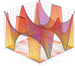The two above curves put together.

Several important Maclaurin series expansions follow.^[8] All these expansions are valid for complex arguments x.

Exponential function:

$e^{x} = \sum^{\infin}_{n=0} \frac{x^n}{n!} = 1 + x + \frac{x^2}{2!} + \frac{x^3}{3!} + \cdots\text{ for all } x\!$

Natural logarithm:

$\log(1-x) = - \sum^{\infin}_{n=1} \frac{x^n}n\text{ for } -1\le x<1$

$\log(1+x) = \sum^{\infin}_{n=1} (-1)^{n+1}\frac{x^n}n\text{ for }-1<x\le1$

Finite geometric series:

$\frac{1-x^{m + 1}}{1-x} = \sum^{m}_{n=0} x^n\quad\mbox{ for } x \not= 1\text{ and } m\in\mathbb{N}_0\!$

Infinite geometric series:

$\frac{1}{1-x} = \sum^{\infin}_{n=0} x^n\text{ for }|x| < 1\!$

Variants of the infinite geometric series:

$\frac{x^m}{1-x} = \sum^{\infin}_{n=m} x^n\quad\mbox{ for }|x| < 1 \text{ and } m\in\mathbb{N}_0\!$

$\frac{x}{(1-x)^2} = \sum^{\infin}_{n=1}n x^n\quad\text{ for }|x| < 1\!$

$\frac{1}{(1-x)^2} = \sum^{\infin}_{n=1}n x^{n-1}\quad\text{ for }|x| < 1\!$

Square root:

$\sqrt{1+x} = \sum_{n=0}^\infty \frac{(-1)^n(2n)!}{(1-2n)(n!)^2(4^n)}x^n = 1 + \textstyle \frac{1}{2}x - \frac{1}{8}x^2 + \frac{1}{16} x^3 - \frac{5}{128} x^4 + \dots\text{ for }|x|\le1$

Binomial series (includes the square root for α = 1/2 and the infinite geometric series for α = −1):

$(1+x)^\alpha = \sum_{n=0}^\infty {\alpha \choose n} x^n\quad\mbox{ for all }|x| < 1 \text{ and all complex } \alpha\!$

with generalized binomial coefficients

${\alpha\choose n} = \prod_{k=1}^n \frac{\alpha-k+1}k = \frac{\alpha(\alpha-1)\cdots(\alpha-n+1)}{n!}$

Trigonometric functions:

$\sin x = \sum^{\infin}_{n=0} \frac{(-1)^n}{(2n+1)!} x^{2n+1} = x - \frac{x^3}{3!} + \frac{x^5}{5!} - \cdots\text{ for all } x\!$

$\cos x = \sum^{\infin}_{n=0} \frac{(-1)^n}{(2n)!} x^{2n} = 1 - \frac{x^2}{2!} + \frac{x^4}{4!} - \cdots\text{ for all } x\!$

$\tan x = \sum^{\infin}_{n=1} \frac{B_{2n} (-4)^n (1-4^n)}{(2n)!} x^{2n-1} = x + \frac{x^3}{3} + \frac{2 x^5}{15} + \cdots\text{ for }|x| < \frac{\pi}{2}\!$

where the B_s are Bernoulli numbers.

$\sec x = \sum^{\infin}_{n=0} \frac{(-1)^n E_{2n}}{(2n)!} x^{2n}\text{ for }|x| < \frac{\pi}{2}\!$

$\arcsin x = \sum^{\infin}_{n=0} \frac{(2n)!}{4^n (n!)^2 (2n+1)} x^{2n+1}\text{ for }|x| \le 1\!$

$\arccos x ={\pi\over 2}-\arcsin x={\pi\over 2}- \sum^{\infin}_{n=0} \frac{(2n)!}{4^n (n!)^2 (2n+1)} x^{2n+1}\text{ for }|x| \le 1\!$

$\arctan x = \sum^{\infin}_{n=0} \frac{(-1)^n}{2n+1} x^{2n+1}\text{ for }|x| \le 1\!$

Hyperbolic functions:

$\sinh x = \sum^{\infin}_{n=0} \frac{x^{2n+1}}{(2n+1)!} = x + \frac{x^3}{3!} + \frac{x^5}{5!} + \cdots\text{ for all } x\!$

$\cosh x = \sum^{\infin}_{n=0} \frac{x^{2n}}{(2n)!} = 1 + \frac{x^2}{2!} + \frac{x^4}{4!} + \cdots\text{ for all } x\!$

$\tanh x = \sum^{\infin}_{n=1} \frac{B_{2n} 4^n (4^n-1)}{(2n)!} x^{2n-1} = x-\frac{1}{3}x^3+\frac{2}{15}x^5-\frac{17}{315}x^7+\cdots \text{ for }|x| < \frac{\pi}{2}\!$

$\mathrm{arsinh} (x) = \sum^{\infin}_{n=0} \frac{(-1)^n (2n)!}{4^n (n!)^2 (2n+1)} x^{2n+1}\text{ for }|x| \le 1\!$

$\mathrm{artanh} (x) = \sum^{\infin}_{n=0} \frac{x^{2n+1}}{2n+1} \text{ for }|x| < 1\!$

Lambert's W function:

$W_0(x) = \sum^{\infin}_{n=1} \frac{(-n)^{n-1}}{n!} x^n\text{ for }|x| < \frac{1}{e}\!$

The numbers B_k appearing in the summation expansions of tan(x) and tanh(x) are the Bernoulli numbers. The E_k in the expansion of sec(x) are Euler numbers.

Calculation of Taylor series

Several methods exist for the calculation of Taylor series of a large number of functions. One can attempt to use the Taylor series as-is and generalize the form of the coefficients, or one can use manipulations such as substitution, multiplication or division, addition or subtraction of standard Taylor series to construct the Taylor series of a function, by virtue of Taylor series being power series. In some cases, one can also derive the Taylor series by repeatedly applying integration by parts. Particularly convenient is the use of computer algebra systems to calculate Taylor series.

First example

Compute the 7^th degree Maclaurin polynomial for the function

$f(x)=\log\cos x, \quad x\in(-\pi/2, \pi/2)\!$.

First, rewrite the function as

$f(x)=\log(1+(\cos x-1))\!$.

We have for the natural logarithm (by using the big O notation)

$\log(1+x) = x - \frac{x^2}2 + \frac{x^3}3 + {O}(x^4)\!$

and for the cosine function

$\cos x - 1 = -\frac{x^2}2 + \frac{x^4}{24} - \frac{x^6}{720} + {O}(x^8)\!$

The latter series expansion has a zero constant term, which enables us to substitute the second series into the first one and to easily omit terms of higher order than the 7^th degree by using the big O notation:

$\begin{align}f(x)&=\log(1+(\cos x-1))\\ &=\bigl(\cos x-1\bigr) - \frac12\bigl(\cos x-1\bigr)^2 + \frac13\bigl(\cos x-1\bigr)^3+ {O}\bigl((\cos x-1)^4\bigr)\\&=\biggl(-\frac{x^2}2 + \frac{x^4}{24} - \frac{x^6}{720} +{O}(x^8)\biggr)-\frac12\biggl(-\frac{x^2}2+\frac{x^4}{24}+{O}(x^6)\biggr)^2+\frac13\biggl(-\frac{x^2}2+O(x^4)\biggr)^3 + {O}(x^8)\\ & =-\frac{x^2}2 + \frac{x^4}{24}-\frac{x^6}{720} - \frac{x^4}8 + \frac{x^6}{48} - \frac{x^6}{24} +O(x^8)\\ & =- \frac{x^2}2 - \frac{x^4}{12} - \frac{x^6}{45}+O(x^8). \end{align}\!$

Since the cosine is an even function, the coefficients for all the odd powers x, x³, x⁵, x⁷, ... have to be zero.

Second example

Suppose we want the Taylor series at 0 of the function

$g(x)=\frac{e^x}{\cos x}\!$.

We have for the exponential function

$e^x = \sum^\infty_{n=0} {x^n\over n!} =1 + x + {x^2 \over 2!} + {x^3 \over 3!} + {x^4 \over 4!}+\cdots\!$

and, as in the first example,

$\cos x = 1 - {x^2 \over 2!} + {x^4 \over 4!} - \cdots\!$

Assume the power series is

${e^x \over \cos x} = c_0 + c_1 x + c_2 x^2 + c_3 x^3 + \cdots\!$

Then multiplication with the denominator and substitution of the series of the cosine yields

$\begin{align} e^x &= (c_0 + c_1 x + c_2 x^2 + c_3 x^3 + \cdots)\cos x\\ &=\left(c_0 + c_1 x + c_2 x^2 + c_3 x^3 + c_4x^4 + \cdots\right)\left(1 - {x^2 \over 2!} + {x^4 \over 4!} - \cdots\right)\\&=c_0 - {c_0 \over 2}x^2 + {c_0 \over 4!}x^4 + c_1x - {c_1 \over 2}x^3 + {c_1 \over 4!}x^5 + c_2x^2 - {c_2 \over 2}x^4 + {c_2 \over 4!}x^6 + c_3x^3 - {c_3 \over 2}x^5 + {c_3 \over 4!}x^7 +\cdots \end{align}\!$

Collecting the terms up to fourth order yields

$=c_0 + c_1x + \left(c_2 - {c_0 \over 2}\right)x^2 + \left(c_3 - {c_1 \over 2}\right)x^3+\left(c_4+{c_0 \over 4!}-{c_2\over 2}\right)x^4 + \cdots\!$

Comparing coefficients with the above series of the exponential function yields the desired Taylor series

$\frac{e^x}{\cos x}=1 + x + x^2 + {2x^3 \over 3} + {x^4 \over 2} + \cdots.\!$

Third example

Here we use a method called "Indirect Expansion" to expand the given function. This method uses the known function of Taylor series for expansion.

Q: Expand the following function as a power series of x

(1 + x)e^x.

We know the Taylor series of function e^x is:

$e^x = \sum^\infty_{n=0} {x^n\over n!} =1 + x + {x^2 \over 2!} + {x^3 \over 3!} + {x^4 \over 4!}+\cdots\!, -\infty<x<+\infty$

Thus,

$\begin{align}(1+x)e^x &= e^x + xe^x = \sum^\infty_{n=0} {x^n\over n!} + \sum^\infty_{n=0} {x^{n+1}\over n!} = 1 + \sum^\infty_{n=1} {x^n\over n!} + \sum^\infty_{n=0} {x^{n+1}\over n!} \\ &= 1 + \sum^\infty_{n=1} {x^n\over n!} + \sum^\infty_{n=1} {x^{n}\over (n-1)!} =1 + \sum^\infty_{n=1}\left({1\over n!} + {1\over (n-1)!}\right)x^n \\ &= 1 + \sum^\infty_{n=1}{n+1\over n!}x^n, -\infty<x<+\infty \\ &= \sum^\infty_{n=0}{n+1\over n!}x^n\end{align}$

Taylor series as definitions

Classically, algebraic functions are defined by an algebraic equation, and transcendental functions (including those discussed above) are defined by some property that holds for them, such as a differential equation. For example, the exponential function is the function which is equal to its own derivative everywhere, and assumes the value 1 at the origin. However, one may equally well define an analytic function by its Taylor series.

Taylor series are used to define functions and "operators" in diverse areas of mathematics. In particular, this is true in areas where the classical definitions of functions break down. For example, using Taylor series, one may define analytical functions of matrices and operators, such as the matrix exponential or matrix logarithm.

In other areas, such as formal analysis, it is more convenient to work directly with the power series themselves. Thus one may define a solution of a differential equation as a power series which, one hopes to prove, is the Taylor series of the desired solution.

Taylor series in several variables

The Taylor series may also be generalized to functions of more than one variable with

$T(x_1,\dots,x_d) =$

$= \sum_{n_1=0}^\infty \cdots \sum_{n_d=0}^\infty \frac{(x_1-a_1)^{n_1}\cdots (x_d-a_d)^{n_d}}{n_1!\cdots n_d!}\,\left(\frac{\partial^{n_1 + \cdots + n_d}f}{\partial x_1^{n_1}\cdots \partial x_d^{n_d}}\right)(a_1,\dots,a_d).\!$

For example, for a function that depends on two variables, x and y, the Taylor series to second order about the point (a, b) is:

$\begin{align} f(x,y) & \approx f(a,b) +(x-a)\, f_x(a,b) +(y-b)\, f_y(a,b) \\ & {}\quad + \frac{1}{2!}\left[ (x-a)^2\,f_{xx}(a,b) + 2(x-a)(y-b)\,f_{xy}(a,b) +(y-b)^2\, f_{yy}(a,b) \right], \end{align}$

where the subscripts denote the respective partial derivatives.

A second-order Taylor series expansion of a scalar-valued function of more than one variable can be written compactly as

$T(\mathbf{x}) = f(\mathbf{a}) + (\mathbf{x} - \mathbf{a})^T\mathrm{D} f(\mathbf{a}) + \frac{1}{2!} (\mathbf{x} - \mathbf{a})^T \,\{\mathrm{D}^2 f(\mathbf{a})\}\,(\mathbf{x} - \mathbf{a}) + \cdots\! \,,$

where $D f(\mathbf{a})\!$ is the gradient of $\,f$ evaluated at $\mathbf{x} = \mathbf{a}$ and $D^2 f(\mathbf{a})\!$ is the Hessian matrix. Applying the multi-index notation the Taylor series for several variables becomes

$T(\mathbf{x}) = \sum_{|\alpha| \ge 0}^{}\frac{(\mathbf{x}-\mathbf{a})^{\alpha}}{\alpha !}\,({\mathrm{\partial}^{\alpha}}\,f)(\mathbf{a})\,,$

which is to be understood as a still more abbreviated multi-index version of the first equation of this paragraph, again in full analogy to the single variable case.

Example

Second-order Taylor series approximation (in gray) of a function f(x,y) = e^xlog (1 + y) around origin.

Compute a second-order Taylor series expansion around point (a,b) = (0,0) of a function

$f(x,y)=e^x\log(1+y).\,$

Firstly, we compute all partial derivatives we need

$f_x(a,b)=e^x\log(1+y)\bigg|_{(x,y)=(0,0)}=0\,,$

$f_y(a,b)=\frac{e^x}{1+y}\bigg|_{(x,y)=(0,0)}=1\,,$

$f_{xx}(a,b)=e^x\log(1+y)\bigg|_{(x,y)=(0,0)}=0\,,$

$f_{yy}(a,b)=-\frac{e^x}{(1+y)^2}\bigg|_{(x,y)=(0,0)}=-1\,,$

$f_{xy}(a,b)=f_{yx}(a,b)=\frac{e^x}{1+y}\bigg|_{(x,y)=(0,0)}=1.$

The Taylor series is

$\begin{align} T(x,y) = f(a,b) & +(x-a)\, f_x(a,b) +(y-b)\, f_y(a,b) \\ &+\frac{1}{2!}\left[ (x-a)^2\,f_{xx}(a,b) + 2(x-a)(y-b)\,f_{xy}(a,b) +(y-b)^2\, f_{yy}(a,b) \right]+ \cdots\,,\end{align}$

which in this case becomes

$\begin{align}T(x,y) &= 0 + 0(x-0) + 1(y-0) + \frac{1}{2}\Big[ 0(x-0)^2 + 2(x-0)(y-0) + (-1)(y-0)^2 \Big] + \cdots \\ &= y + xy - \frac{y^2}{2} + \cdots. \end{align}$

Since log(1 + y) is analytic in |y| < 1, we have

$e^x\log(1+y)= y + xy - \frac{y^2}{2} + \cdots$

for |y| < 1.

Fractional Taylor series

With the emergence of fractional calculus, a natural question arises about what the Taylor Series expansion would be. Odibat and Shawagfeh^[9] answered this in 2007. By using the Caputo fractional derivative, $0<\alpha<1\,\!$, and $x+\,\!$ indicating the limit as we approach $x\,\!$ from the right, the fractional Taylor series can be written as

$f(x+\Delta x) = f(x) + D_x^\alpha f(x+)\frac{(\Delta x)^\alpha}{\Gamma(\alpha+1)} + D_x^\alpha D_x^\alpha f(x+)\frac{(\Delta x)^{2\alpha}}{\Gamma(2\alpha+1)} + \cdots.$

See also

• Taylor's theorem
• Linear approximation
• Laurent series
• Analyticity of holomorphic functions — a proof that a holomorphic function can be expressed as a Taylor power series
• Newton's divided difference interpolation
• Difference engine
• Mean value theorem
• Madhava series

Notes

1. ^ Kline, M. (1990) Mathematical Thought from Ancient to Modern Times. Oxford University Press. pp. 35-37.
2. ^ Boyer, C. and Merzbach, U. (1991) A History of Mathematics. John Wiley and Sons. pp. 202-203.
3. ^ "Neither Newton nor Leibniz - The Pre-History of Calculus and Celestial Mechanics in Medieval Kerala". MAT 314. Canisius College. http://www.canisius.edu/topos/rajeev.asp. Retrieved 2006-07-09. 
4. ^ Taylor, Brook, Methodus Incrementorum Directa et Inversa [Direct and Reverse Methods of Incrementation] (London, 1715), pages 21-23 (Proposition VII, Theorem 3, Corollary 2). Translated into English in D. J. Struik, A Source Book in Mathematics 1200-1800 (Cambridge, Massachusetts: Harvard University Press, 1969), pages 329-332.
5. ^ Rudin, Walter (1980), Real and Complex Analysis, New Dehli: McGraw-Hill, p. 418, Exercise 13, ISBN 0-07-099557-5 
6. ^ Feller, William (1971), An introduction to probability theory and its applications, Volume 2 (3rd ed.), Wiley, pp. 230–232 .
7. ^ Hille, Einar; Phillips, Ralph S. (1957), Functional analysis and semi-groups, AMS Colloquium Publications, 31, American Mathematical Society, p. 300–327 .
8. ^ Most of these can be found in (Abramowitz & Stegun 1970).
9. ^ Odibat, ZM., Shawagfeh, NT., 2007. "Generalized Taylor's formula." Applied Mathematics and Computation 186, 286-293.

References

• Abramowitz, Milton; Stegun, Irene A. (1970), Handbook of Mathematical Functions with Formulas, Graphs, and Mathematical Tables, New York: Dover Publications, Ninth printing 
• Thomas, George B. Jr.; Finney, Ross L. (1996), Calculus and Analytic Geometry (9th ed.), Addison Wesley, ISBN 0-201-53174-7 
• Greenberg, Michael (1998), Advanced Engineering Mathematics (2nd ed.), Prentice Hall, ISBN 0-13-321431-1 

External links

• Weisstein, Eric W., "Taylor Series" from MathWorld.
• Madhava of Sangamagramma
• Taylor Series Representation Module by John H. Mathews
• "Discussion of the Parker-Sochacki Method"
• Another Taylor visualisation - where you can choose the point of the approximation and the number of derivatives
• Taylor series revisited for numerical methods at Numerical Methods for the STEM Undergraduate
• Cinderella 2: Taylor expansion
• Taylor series
• Inverse trigonometric functions Taylor series