Runge's phenomenon

---

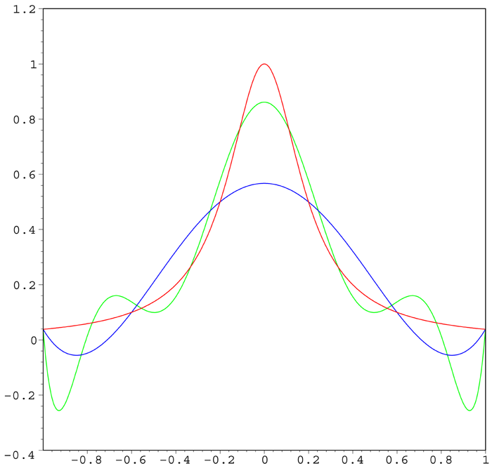
right|thumb|300px|The red curve is ">red|the Runge function. The blue curve is blue|a 5th-order interpolating polynomial (using six equally-spaced interpolating points). The green curve is green|a 9th-order interpolating polynomial (using ten equally-spaced interpolating points). At the interpolating points, the error between the function and the interpolating polynomial is (by definition) zero. Between the interpolating points (especially in the region close to the endpoints 1 and −1), the error between the function and the interpolating polynomial gets worse for higher-order polynomials.

In the mathematical field of numerical analysis, Runge's phenomenon is a problem that occurs when using polynomial interpolation with polynomials of high degree. It was discovered by Carl David Tolmé Runge when exploring the behavior of errors when using polynomial interpolation to approximate certain functions harv|Runge|1901.

Problem

Consider the function:

:$f(x)\; =\; frac\{1\}\{1+25x^2\}.,$

Runge found that if this function is interpolated at equidistant points "x"_"i" between −1 and 1 such that:

:$x\_i\; =\; -1\; +\; (i-1)frac\{2\}\{n\},quad\; i\; in\; left\{\; 1,\; 2,\; dots,\; n+1\; ight\}$

with a polynomial "P"_"n"("x") of degree ≤ "n", the resulting interpolation oscillates toward the end of the interval, i.e. close to −1 and 1. It can even be proven that the interpolation error tends toward infinity when the degree of the polynomial increases:

:$lim\_\{n\; ightarrow\; infty\}\; left(\; max\_\{-1\; leq\; x\; leq\; 1\}\; |\; f(x)\; -P\_n(x)|\; ight)\; =\; infty.$

However, the Weierstrass approximation theorem states that there is some sequence of approximating polynomials for which the error goes to zero. This shows that high-degree polynomial interpolation at equidistant points can be troublesome.

Reason

The error between the generating function and the interpolating polynomial of order "N" is bounded by the "N"th derivative of the generating function.

For the case of the Runge function (also called the Cauchy-Lorentz function) shown above,:$f(x)\; =\; frac\{1\}\{1+25x^2\}$the first two derivatives are:The magnitude of higher order derivatives of the Runge function get even larger. Therefore, the bound for the error (between the interpolating points) when using higher order interpolating polynomials becomes larger.

Mitigations to the problem of Runge's phenomenon

The oscillation can be minimized by using nodes that are distributed more densely towards the edges of the interval, specifically, with asymptotic density (on the interval [-1,1] ) given by$1/sqrt\{1-x^2\}$harv|Berrut|Trefethen|2004.A standard example of such a set of nodes is Chebyshev nodes, for which the maximum error is guaranteed to diminish with increasing polynomial order. The phenomenon demonstrates that high degree polynomials are generally unsuitable for interpolation with equidistant nodes. The problem can be avoided by using spline curves which are piecewise polynomials. When trying to decrease the interpolation error one can increase the number of polynomial pieces which are used to construct the spline instead of increasing the degree of the polynomials used.

See also

* Compare with the Gibbs phenomenon for sinusoidal basis functions

References

*.
*