Numerical stability

In the mathematical subfield of numerical analysis, numerical stability is a desirable property of numerical algorithms. The precise definition of stability depends on the context, but it is related to the accuracy of the algorithm.

A related phenomenon is instability. Typically, algorithms would approach the right solution in the limit, if there were no round-off or truncation errors, but depending on the specific computational method, errors can be magnified, instead of damped, causing the error to grow exponentially.

Sometimes a single calculation can be achieved in several ways, all of which are algebraically equivalent in terms of ideal real or complex numbers, but in practice when performed on digital computers yield different results. Some calculations might damp out approximation errors that occur; others might magnify such errors. Calculations that can be proven not to magnify approximation errors are called numerically stable. One of the common tasks of numerical analysis is to try to select algorithms which are robust — that is to say, have good numerical stability among other desirable properties.

Example

As an example of an unstable algorithm, consider the task of adding an array of 100 numbers. To simplify things, assume our computer only has two digits of precision (for example, numbers can be represented as 2.3, 77, 100, 110, 120, etc., but not 12.3 or 177).

The naive way to do this would be the following:

function sumArray(array) is
    let theSum = 0
    for each element in array do
        let theSum = theSum + element
    end for
    return theSum
 end function

That looks reasonable, but suppose the first element in the array was 1.0 and the other 99 elements were 0.01. In exact arithmetic, the answer would be 1.99. However, on our two-digit computer, once the 1.0 was added into the sum variable, adding in 0.01 would have no effect on the sum, and so the final answer would be 1.0 – not a very good approximation of the real answer. Furthermore, we see that the algorithm depends on the ordering of elements within the array, in contrast to the exact arithmetic.

A stable algorithm would first sort the array by the absolute values of the elements in ascending order. This ensures that the numbers closest to zero will be taken into consideration first. Once that change is made, all of the 0.01 elements will be added, giving 0.99, and then the 1.0 element will be added, yielding a rounded result of 2.0 – a much better approximation of the real result.

Forward, backward, and mixed stability

There are different ways to formalize the concept of stability. The following definitions of forward, backward, and mixed stability are often used in numerical linear algebra.

Diagram showing the forward error Δy and the backward error Δx, and their relation to the exact solution map f and the numerical solution f*.

Consider the problem to be solved by the numerical algorithm as a function f mapping the data x to the solution y. The result of the algorithm, say y*, will usually deviate from the "true" solution y. The main causes of error are round-off error and truncation error. The forward error of the algorithm is the difference between the result and the solution; in this case, Δy = y* − y. The backward error is the smallest Δx such that f(x + Δx) = y*; in other words, the backward error tells us what problem the algorithm actually solved. The forward and backward error are related by the condition number: the forward error is at most as big in magnitude as the condition number multiplied by the magnitude of the backward error.

In many cases, it is more natural to consider the relative error

$\frac{|\Delta x|}{|x|}$

instead of the absolute error Δx.

The algorithm is said to be backward stable if the backward error is small for all inputs x. Of course, "small" is a relative term and its definition will depend on the context. Often, we want the error to be of the same order as, or perhaps only a few orders of magnitude bigger than, the unit round-off.

Mixed stability combines the concepts of forward error and backward error.

The usual definition of numerical stability uses a more general concept, called mixed stability, which combines the forward error and the backward error. An algorithm is stable in this sense if it solves a nearby problem approximately, i.e., if there exists a Δx such that both Δx is small and f(x + Δx) − y* is small. Hence, a backward stable algorithm is always stable.

An algorithm is forward stable if its forward error divided by the condition number of the problem is small. This means that an algorithm is forward stable if it has a forward error of magnitude similar to some backward stable algorithm.

Error growth

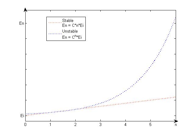
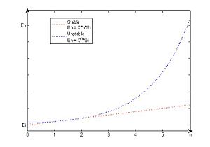Comparing the linear error growth of a stable algorithm and the exponential error growth of an unstable algorithm used to solve the same problem, with the same initial data.

Definition

Suppose that E_i > 0 denotes an initial error and E_n represents the magnitude of an error after n subsequent operations. If E_n ≈ C*n*E_i, where C is a constant independent of n, then the growth of the error is said to be linear. If E_n ≈ Cⁿ*E_i, for some C > 1, then the growth of the error is called exponential.

Stability in numerical differential equations

The above definitions are particularly relevant in situations where truncation errors are not important. In other contexts, for instance when solving differential equations, a different definition of numerical stability is used.

In numerical ordinary differential equations, various concepts of numerical stability exist, for instance A-stability. They are related to some concept of stability in the dynamical systems sense, often Lyapunov stability. It is important to use a stable method when solving a stiff equation.

Yet another definition is used in numerical partial differential equations. An algorithm for solving a linear evolutionary partial differential equation is stable if the total variation of the numerical solution at a fixed time remains bounded as the step size goes to zero. The Lax equivalence theorem states that an algorithm converges if it is consistent and stable (in this sense). Stability is sometimes achieved by including numerical diffusion. Numerical diffusion is a mathematical term which ensures that roundoff and other errors in the calculation get spread out and do not add up to cause the calculation to "blow up". von Neumann stability analysis is a commonly used procedure for the stability analysis of finite difference schemes as applied to linear partial differential equations. These results do not hold for nonlinear PDEs, where a general, consistent definition of stability is complicated by many properties absent in linear equations.

See also

• Algorithms for calculating variance

References

• Nicholas J. Higham, Accuracy and Stability of Numerical Algorithms, Society of Industrial and Applied Mathematics, Philadelphia, 1996. ISBN 0-89871-355-2.
• Richard L. Burden and J. Douglas Faires, Numerical Analysis 8th Edition, Thomson Brooks/Cole, U.S., 2005. ISBN 0-534-39200-8