Numerical ordinary differential equations

Illustration of numerical integration for the differential equation y' = y,y(0) = 1. Blue: the Euler method, green: the midpoint method, red: the exact solution, y = e^t. The step size is h = 1.0.

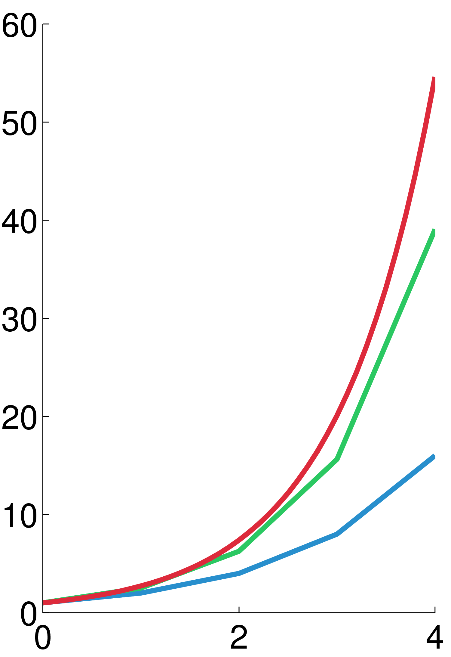
The same illustration for h = 0.25. It is seen that the midpoint method converges faster than the Euler method.

Numerical ordinary differential equations is the part of numerical analysis which studies the numerical solution of ordinary differential equations (ODEs). This field is also known under the name numerical integration, but some people reserve this term for the computation of integrals.

Many differential equations cannot be solved analytically; however, in science and engineering, a numeric approximation to the solution is often good enough to solve a problem. The algorithms studied here can be used to compute such an approximation. An alternative method is to use techniques from calculus to obtain a series expansion of the solution.

Ordinary differential equations occur in many scientific disciplines, for instance in physics, chemistry, biology, and economics. In addition, some methods in numerical partial differential equations convert the partial differential equation into an ordinary differential equation, which must then be solved.

The problem

We want to approximate the solution of the differential equation

$y'(t) = f(t,y(t)), \qquad y(t_0)=y_0, \qquad\qquad (1)$

where f is a function that maps [t₀,∞) × R^d to R^d, and the initial condition y₀ ∈ R^d is a given vector.

The above formulation is called an initial value problem (IVP). The Picard–Lindelöf theorem states that there is a unique solution, if f is Lipschitz continuous. In contrast, boundary value problems (BVPs) specify (components of) the solution y at more than one point. Different methods need to be used to solve BVPs, for example the shooting method (and its variants) or global methods like finite differences, Galerkin methods, or collocation methods.

Note that we restrict ourselves to first-order differential equations (meaning that only the first derivative of y appears in the equation, and no higher derivatives). However, a higher-order equation can easily be converted to a system of first-order equations by introducing extra variables. For example, the second-order equation y'' = −y can be rewritten as two first-order equations: y' = z and z' = −y.

Methods

Three elementary methods are discussed to give the reader a feeling for the subject. After that, pointers are provided to other methods (which are generally more accurate and efficient). The methods mentioned here are analysed in the next section.

The Euler method

For more details on this topic, see Euler method.

A brief explanation: From any point on a curve, you can find an approximation of a nearby point on the curve by moving a short distance along a line tangent to the curve.

Rigorous development: Starting with the differential equation (1), we replace the derivative y' by the finite difference approximation

$y'(t) \approx \frac{y(t+h) - y(t)}{h}, \qquad\qquad (2)$

which when re-arranged yields the following formula

$y(t+h) \approx y(t) + hy'(t) \qquad\qquad$

and using (1) gives:

$y(t+h) \approx y(t) + hf(t,y(t)). \qquad\qquad (3)$

This formula is usually applied in the following way. We choose a step size h, and we construct the sequence t₀, t₁ = t₀ + h, t₂ = t₀ + 2h, … We denote by y_n a numerical estimate of the exact solution y(t_n). Motivated by (3), we compute these estimates by the following recursive scheme

$y_{n+1} = y_n + hf(t_n,y_n). \qquad\qquad (4)$

This is the Euler method (or forward Euler method, in contrast with the backward Euler method, to be described below). The method is named after Leonhard Euler who described it in 1768.

The Euler method is an example of an explicit method. This means that the new value y_n+1 is defined in terms of things that are already known, like y_n.

The backward Euler method

If, instead of (2), we use the approximation

$y'(t) \approx \frac{y(t) - y(t-h)}{h}, \qquad\qquad (5)$

we get the backward Euler method:

$y_{n+1} = y_n + hf(t_{n+1},y_{n+1}). \qquad\qquad (6)$

The backward Euler method is an implicit method, meaning that we have to solve an equation to find y_n+1. One often uses fixed point iteration or (some modification of) the Newton–Raphson method to achieve this. Of course, it costs time to solve this equation; this cost must be taken into consideration when one selects the method to use. The advantage of implicit methods such as (6) is that they are usually more stable for solving a stiff equation, meaning that a larger step size h can be used.

The exponential Euler method

If the differential equation is of the form

$y'(t) = A-By(t) \qquad\qquad\qquad (7)$

then an approximate explicit solution can be given by

$y_{n+1} = y_n e^{-Bh}+\frac{A}{B}(1-e^{-Bh})\ . \qquad\qquad (8)$

This method is commonly employed in neural simulations and it is the default integrator in the GENESIS neural simulator.^[1]

Generalizations

The Euler method is often not accurate enough. In more precise terms, it only has order one (the concept of order is explained below). This caused mathematicians to look for higher-order methods.

One possibility is to use not only the previously computed value y_n to determine y_n+1, but to make the solution depend on more past values. This yields a so-called multistep method. Perhaps the simplest is the Leapfrog method which is second order and (roughly speaking) relies on two time values.

Almost all practical multistep methods fall within the family of linear multistep methods, which have the form

$\alpha_k y_{n+k} + \alpha_{k-1} y_{n+k-1} + \cdots + \alpha_0 y_n$

$= h \left[ \beta_k f(t_{n+k},y_{n+k}) + \beta_{k-1} f(t_{n+k-1},y_{n+k-1}) + \cdots + \beta_0 f(t_n,y_n) \right].$

Another possibility is to use more points in the interval [t_n,t_n+1]. This leads to the family of Runge–Kutta methods, named after Carl Runge and Martin Kutta. One of their fourth-order methods is especially popular.

Advanced features

A good implementation of one of these methods for solving an ODE entails more than the time-stepping formula.

It is often inefficient to use the same step size all the time, so variable step-size methods have been developed. Usually, the step size is chosen such that the (local) error per step is below some tolerance level. This means that the methods must also compute an error indicator, an estimate of the local error.

An extension of this idea is to choose dynamically between different methods of different orders (this is called a variable order method). Methods based on Richardson extrapolation, such as the Bulirsch–Stoer algorithm, are often used to construct various methods of different orders.

Other desirable features include:

• dense output: cheap numerical approximations for the whole integration interval, and not only at the points t₀, t₁, t₂, ...
• event location: finding the times where, say, a particular function vanishes. This typically requires the use of a root-finding algorithm.
• support for parallel computing.
• when used for integrating with respect to time, time reversibility

Alternative methods

Many methods do not fall within the framework discussed here. Some classes of alternative methods are:

• multiderivative methods, which use not only the function f but also its derivatives. This class includes Hermite–Obreschkoff methods and Fehlberg methods, as well as methods like the Parker–Sochacki method or Bychkov-Scherbakov method, which compute the coefficients of the Taylor series of the solution y recursively.
• methods for second order ODEs. We said that all higher-order ODEs can be transformed to first-order ODEs of the form (1). While this is certainly true, it may not be the best way to proceed. In particular, Nyström methods work directly with second-order equations.
• geometric integration methods are especially designed for special classes of ODEs (e.g., symplectic integrators for the solution of Hamiltonian equations). They take care that the numerical solution respects the underlying structure or geometry of these classes.

Analysis

Numerical analysis is not only the design of numerical methods, but also their analysis. Three central concepts in this analysis are:

• convergence: whether the method approximates the solution,
• order: how well it approximates the solution, and
• stability: whether errors are damped out.

Convergence

A numerical method is said to be convergent if the numerical solution approaches the exact solution as the step size h goes to 0. More precisely, we require that for every ODE (1) with a Lipschitz function f and every t^* > 0,

$\lim_{h\to0+} \max_{n=0,1,\dots,\lfloor t^*/h\rfloor} \| y_{n,h} - y(t_n) \| = 0.$

All the methods mentioned above are convergent. In fact, convergence is a condition sine qua non for any numerical scheme.

Consistency and order

Suppose the numerical method is

$y_{n+k} = \Psi(t_{n+k}; y_n, y_{n+1}, \dots, y_{n+k-1}; h). \,$

The local error of the method is the error committed by one step of the method. That is, it is the difference between the result given by the method, assuming that no error was made in earlier steps, and the exact solution:

$\delta^h_{n+k} = \Psi \left( t_{n+k}; y(t_n), y(t_{n+1}), \dots, y(t_{n+k-1}); h \right) - y(t_{n+k}).$

The method is said to be consistent if

$\lim_{h\to 0} \frac{\delta^h_{n+k}}{h} = 0.$

The method has order p if

$\delta^h_{n+k} = O(h^{p+1}) \quad\mbox{as } h\to0.$

Hence a method is consistent if it has an order greater than 0. The (forward) Euler method (4) and the backward Euler method (6) introduced above both have order 1, so they are consistent. Most methods being used in practice attain higher order. Consistency is a necessary condition for convergence, but not sufficient; for a method to be convergent, it must be both consistent and zero-stable.

A related concept is the global error, the error sustained in all the steps one needs to reach a fixed time t. Explicitly, the global error at time t is y_N − y(t) where N = (t−t₀)/h. The global error of a pth order one-step method is O(h^p); in particular, such a method is convergent. This statement is not necessarily true for multi-step methods.

Stability and stiffness

Main article: Stiff equation

For some differential equations, application of standard methods—such as the Euler method, explicit Runge–Kutta methods, or multistep methods (e.g., Adams–Bashforth methods)—exhibit instability in the solutions, though other methods may produce stable solutions. This "difficult behaviour" in the equation (which may not necessarily be complex itself) is described as stiffness, and is often caused by the presence of different time scales in the underlying problem. Stiff problems are ubiquitous in chemical kinetics, control theory, solid mechanics, weather forecasting, biology, plasma physics, and electronics.

History

Below is a timeline of some important developments in this field.

• 1768 - Leonhard Euler publishes his method.
• 1824 - Augustin Louis Cauchy proves convergence of the Euler method. In this proof, Cauchy uses the implicit Euler method.
• 1855 - First mention of the multistep methods of John Couch Adams in a letter written by F. Bashforth.
• 1895 - Carl Runge publishes the first Runge–Kutta method.
• 1905 - Martin Kutta describes the popular fourth-order Runge–Kutta method.
• 1910 - Lewis Fry Richardson announces his extrapolation method, Richardson extrapolation.
• 1952 - Charles F. Curtiss and Joseph Oakland Hirschfelder coin the term stiff equations.

See also

• Courant–Friedrichs–Lewy condition
• Energy drift
• List of numerical analysis topics#Numerical ordinary differential equations
• Reversible reference system propagation algorithm
• Trapezoidal rule

Software for ODE solving

• MATLAB
• FuncDesigner (free license: BSD, uses Automatic differentiation, also can be used online via Sage-server)
• VisSim - a visual language for differential equation solving
• Mathematical Assistant on Web online solving first order (linear and with separated variables) and second order linear differential equations (with constant coefficients), including intermediate steps in the solution.
• DotNumerics: Ordinary Differential Equations for C# and VB.NET Initial-value problem for nonstiff and stiff ordinary differential equations (explicit Runge-Kutta, implicit Runge-Kutta, Gear’s BDF and Adams-Moulton).
• Online experiments with JSXGraph
• Maxima computer algebra system (GPL)

References

1. ^ http://www.genesis-sim.org/BABEL/gum-tutorials/cornelis/doc/html/node9.html

• J. C. Butcher, Numerical methods for ordinary differential equations, ISBN 0471967580
• Ernst Hairer, Syvert Paul Nørsett and Gerhard Wanner, Solving ordinary differential equations I: Nonstiff problems, second edition, Springer Verlag, Berlin, 1993. ISBN 3-540-56670-8.
• Ernst Hairer and Gerhard Wanner, Solving ordinary differential equations II: Stiff and differential-algebraic problems, second edition, Springer Verlag, Berlin, 1996. ISBN 3-540-60452-9.
  (This two-volume monograph systematically covers all aspects of the field.)
• Arieh Iserles, A First Course in the Numerical Analysis of Differential Equations, Cambridge University Press, 1996. ISBN 0-521-55376-8 (hardback), ISBN 0-521-55655-4 (paperback).
  (Textbook, targeting advanced undergraduate and postgraduate students in mathematics, which also discusses numerical partial differential equations.)
• John Denholm Lambert, Numerical Methods for Ordinary Differential Systems, John Wiley & Sons, Chichester, 1991. ISBN 0-471-92990-5.
  (Textbook, slightly more demanding than the book by Iserles.)

External links

• Joseph W. Rudmin, Application of the Parker–Sochacki Method to Celestial Mechanics, 1998.
• Dominique Tournès, L'intégration approchée des équations différentielles ordinaires (1671-1914), thèse de doctorat de l'université Paris 7 - Denis Diderot, juin 1996. Réimp. Villeneuve d'Ascq : Presses universitaires du Septentrion, 1997, 468 p. (Extensive online material on ODE numerical analysis history, for English-language material on the history of ODE numerical analysis, see e.g. the paper books by Chabert and Goldstine quoted by him.)