Isoperimetric inequality

The isoperimetric inequality is a geometric inequality involving the square of the circumference of a closed curve in the plane and the area of a plane region it encloses, as well as its various generalizations. Isoperimetric literally means "having the same perimeter". Specifically, the isoperimetric inequality states, for the length L of a closed curve and the area A of the planar region that it encloses, that

$4\pi A \le L^2,$

and that equality holds if and only if the curve is a circle.

The isoperimetric problem is to determine a plane figure of the largest possible area whose boundary has a specified length. The closely related Dido's problem asks for a region of the maximal area bounded by a straight line and a curvilinear arc whose endpoints belong to that line. It is named after Dido, the legendary founder and first queen of Carthage. The solution to the isoperimetric problem is given by a circle and was known already in Ancient Greece. However, the first mathematically rigorous proof of this fact was obtained only in the 19th century. Since then, many other proofs have been found, some of them stunningly simple. The isoperimetric problem has been extended in multiple ways, for example, to curves on surfaces and to regions in higher-dimensional spaces.

Perhaps the most familiar physical manifestation of the 3-dimensional isoperimetric inequality is the shape of a drop of water. Namely, a drop will typically assume a symmetric round shape. Since the amount of water in a drop is fixed, surface tension forces the drop into a shape which minimizes the surface area of the drop, namely a round sphere.

The isoperimetric problem in the plane

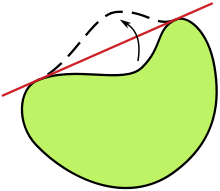If a region is not convex, a "dent" in its boundary can be "flipped" to increase the area of the region while keeping the perimeter unchanged.

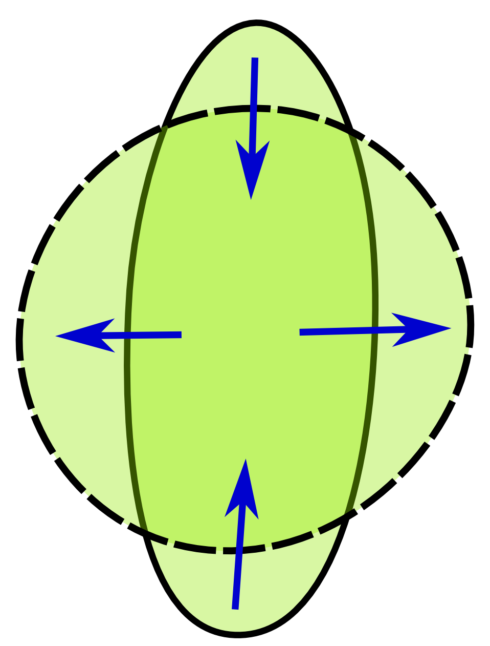
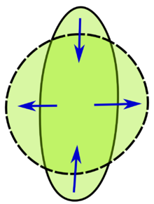An elongated shape can be made more round while keeping its perimeter fixed and increasing its area.

The classical isoperimetric problem dates back to antiquity. The problem can be stated as follows: Among all closed curves in the plane of fixed perimeter, which curve (if any) maximizes the area of its enclosed region? This question can be shown to be equivalent to the following problem: Among all closed curves in the plane enclosing a fixed area, which curve (if any) minimizes the perimeter?

This problem is conceptually related to the principle of least action in physics, in that it can be restated: what is the principle of action which encloses the greatest area, with the greatest economy of effort? The 15th-century philosopher and scientist, Cardinal Nicholas of Cusa, considered rotational action, the process by which a circle is generated, to be the most direct reflection, in the realm of sensory impressions, of the process by which the universe is created. German astronomer and astrologer Johannes Kepler invoked the isoperimetric principle in discussing the morphology of the solar system, in Mysterium Cosmographicum (The Sacred Mystery of the Cosmos, 1596).

Although the circle appears to be an obvious solution to the problem, proving this fact is rather difficult. The first progress toward the solution was made by Swiss geometer Jakob Steiner in 1838, using a geometric method later named Steiner symmetrisation.^[1] Steiner showed that if a solution existed, then it must be the circle. Steiner's proof was completed later by several other mathematicians.

Steiner begins with some geometric constructions which are easily understood; for example, it can be shown that any closed curve enclosing a region that is not fully convex can be modified to enclose more area, by "flipping" the concave areas so that they become convex. It can further be shown that any closed curve which is not fully symmetrical can be "tilted" so that it encloses more area. The one shape that is perfectly convex and symmetrical is the circle, although this, in itself, does not represent a rigorous proof of the isoperimetric theorem (see external links).

The isoperimetric inequality

The solution to the isoperimetric problem is usually expressed in the form of an inequality that relates the length L of a closed curve and the area A of the planar region that it encloses. The isoperimetric inequality states that

$4\pi A \le L^2,$

and that the equality holds if and only if the curve is a circle. Indeed, the area of a disk of radius R is πR² and the circumference of the circle is 2πR, so both sides of the inequality are equal to 4π²R² in this case.

Dozens of proofs of the isoperimetric inequality have been found. In 1902, Hurwitz published a short proof using the Fourier series that applies to arbitrary rectifiable curves (not assumed to be smooth). An elegant direct proof based on comparison of a smooth simple closed curve with an appropriate circle was given by E. Schmidt in 1938. It uses only the arc length formula, expression for the area of a plane region from Green's theorem, and the Cauchy–Schwarz inequality.

For a given closed curve, the isoperimetric quotient is defined as the ratio of its area and that of the circle having the same perimeter. This is equal to

$Q=\frac{4\pi A}{L^2}$

and the isoperimetric inequality says that Q ≤ 1.

The isoperimetric quotient of a regular n-gon is

$Q_n=\frac{\pi}{n \tan \tfrac{\pi}{n}}$.

The isoperimetric inequality on the sphere

Let C be a simple closed curve on a sphere of radius 1. Denote by L the length of C and by A the area enclosed by C. The spherical isoperimetric inequality states that

$L^2 \, \ge \, A (4\pi - A),$

and that the equality holds if and only if the curve is a circle. There are, in fact, two ways to measure the spherical area enclosed by a simple closed curve, but the inequality is symmetric with the respect to taking the complement.

This inequality was discovered by Paul Lévy (1919) who also extended it to higher dimensions and general surfaces.

Isoperimetric inequality in higher dimensions

The isoperimetric theorem generalizes to surfaces in the three-dimensional Euclidean space. Among all simple closed surfaces with given surface area, the sphere encloses a region of maximal volume. An analogous statement holds in Euclidean spaces of any dimension.

In full generality (Federer 1969, §3.2.43), the isoperimetric inequality states that for any set S ⊂ Rⁿ whose closure has finite Lebesgue measure

$n\omega_n^{1/n} L^n(\bar{S})^{(n-1)/n} \le M^{n-1}_*(\partial S)$

where M_*^n-1 is the (n-1)-dimensional Minkowski content, Lⁿ is the n-dimensional Lebesgue measure, and ω_n is the volume of the unit ball in Rⁿ. If the boundary of S is rectifiable, then the Minkowski content is the (n-1)-dimensional Hausdorff measure.

The isoperimetric inequality in n-dimensions can be quickly proven by the Brunn-Minkowski inequality (Osserman (1978); Federer (1969, §3.2.43)).

The n-dimensional isoperimetric inequality is equivalent (for sufficiently smooth domains) to the Sobolev inequality on Rⁿ with optimal constant:

$\left(\int_{\mathbb{R}^n} |u|^{\frac{n}{n-1}}\right)^{\frac{n-1}{n}} \le n^{-1}\omega_n^{-1/n}\int_{\mathbb{R}^n}|\nabla u|$

for all u ∈ W^1,1(Rⁿ).

Isoperimetric inequalities in a metric measure space

Most of the work on isoperimetric problem has been done in the context of smooth regions in Euclidean spaces, or more generally, in Riemannian manifolds. However, the isoperimetric problem can be formulated in much greater generality, using the notion of Minkowski content. Let $\scriptstyle(X,\, \mu,\, d)$ be a metric measure space: X is a metric space with metric d, and μ is a Borel measure on X. The boundary measure, or Minkowski content, of a measurable subset A of X is defined as the lim inf

$\mu^+(A) = \liminf_{\varepsilon \to 0+} \frac{\mu(A_\varepsilon) - \mu(A)}{2\varepsilon},$

where

$A_\varepsilon = \{ x \in X \, | \, d(x, A) \leq \varepsilon \}$

is the ε-extension of A.

The isoperimetric problem in X asks how small can $\scriptstyle\mu^+(A)$ be for a given μ(A). If X is the Euclidean plane with the usual distance and the Lebesgue measure then this question generalizes the classical isoperimetric problem to planar regions whose boundary is not necessarily smooth, although the answer turns out to be the same.

The function

$I(a) \,=\, \inf \{ \mu^+(A) \, | \, \mu(A)\, =\, a\}$

is called the isoperimetric profile of the metric measure space $\scriptstyle(X,\, \mu,\, d)$. Isoperimetric profiles have been studied for Cayley graphs of discrete groups and for special classes of Riemannian manifolds (where usually only regions A with regular boundary are considered).

Isoperimetric inequalities for Graphs

Main article: Expander graph

In graph theory, isoperimetric inequalities are at the heart of the study of expander graphs, which are sparse graphs that have strong connectivity properties. Expander constructions have spawned research in pure and applied mathematics, with several applications to complexity theory, design of robust computer networks, and the theory of error-correcting codes.^[2]

Isoperimetric inequalities for graphs relate the size of vertex subsets to the size of their boundary, which is usually measured by the number of edges leaving the subset (edge expansion) or by the number of neighbouring vertices (vertex expansion). For a graph G and a number k, the following are two standard isoperimetric parameters for graphs.^[3]

The edge isoperimetric parameter: $\Phi_E(G,k)=\min_{S\subseteq V} \left\{|E(S,\overline{S})| : |S|=k \right\}$

The vertex isoperimetric parameter: $\Phi_V(G,k)=\min_{S\subseteq V} \left\{|\Gamma(S)\setminus S| : |S|=k \right\}$

Here $E(S,\overline{S})$ denotes the set of edges leaving S and Γ(S) denotes the set of vertices that have a neighbour in S. The isoperimetric problem consists of understanding how the parameters Φ_E and Φ_V behave for natural families of graphs.

Example: Isoperimetric inequalities for hypercubes

The d-dimensional hypercube Q_d is the graph whose vertices are all Boolean vectors of length d, that is, the set {0,1}^d. Two such vectors are connected by an edge in Q_d if they are equal up to a single bit flip, that is, their Hamming distance is exactly one. The following are the isoperimetric inequalities for the Boolean hypercube.^[4]

Edge isoperimetric inequality

The edge isoperimetric inequality of the hypercube is $\Phi_E(Q_d,k) \geq k(d-\log_2 k)$. This bound is tight, as is witnessed by each set S that is the set of vertices of any subcube of Q_d.

Vertex isoperimetric inequality

Harper's theorem^[5] says that Hamming balls have the smallest vertex boundary among all sets of a given size. Hamming balls are sets that contain all points of Hamming weight at most r and no points of Hamming weight larger than r + 1 for some integer r. This theorem implies that any set $S\subseteq V$ with $|S|\geq\sum_{i=0}^{r} {n\choose i}$ satisfies $|S\cup\Gamma(S)|\geq \sum_{i=0}^{r+1}{n\choose i}$.^[6]

As a special case, consider set sizes k = | S | of the form $k={d \choose 0} + {d \choose 1} + \dots + {d \choose r}$ for some integer r. Then the above implies that the exact vertex isoperimetric parameter is $\Phi_V(Q_d,k) = {d\choose r+1}$.^[7]

See also

• Isoperimetric dimension
• Chaplygin problem
• Gaussian isoperimetric inequality
• Lévy–Gromov inequality
• Expander graph
• Planar separator theorem

Notes

1. ^ J. Steiner, Einfacher Beweis der isoperimetrischen Hauptsätze, J. reine angew Math. 18, (1838), pp. 281–296; and Gesammelte Werke Vol. 2, pp. 77–91, Reimer, Berlin, (1882).
2. ^ Hoory, Linial & Widgerson (2006)
3. ^ Definitions 4.2 and 4.3 of Hoory, Linial & Widgerson (2006)
4. ^ See Bollobás (1986) and Section 4 in Hoory, Linial & Widgerson (2006)
5. ^ Cf. Calabro (2004) or Bollobás (1986)
6. ^ cf. Leader (1991)
7. ^ Also stated in Hoory, Linial & Widgerson (2006)

References

• Blaschke and Leichtweiß, Elementare Differentialgeometrie (in German), 5th edition, completely revised by K. Leichtweiß. Die Grundlehren der mathematischen Wissenschaften, Band 1. Springer-Verlag, New York Heidelberg Berlin, 1973 ISBN 0-387-05889-3
• Bollobás, Béla (1986). Combinatorics: set systems, hypergraphs, families of vectors, and combinatorial probability. Cambridge University Press. ISBN 9780521337038 
• Burago (2001), "Isoperimetric inequality", in Hazewinkel, Michiel, Encyclopaedia of Mathematics, Springer, ISBN 978-1556080104, http://eom.springer.de/I/i052860.htm 
• Calabro, Chris (2004). "Harper's Theorem". http://cseweb.ucsd.edu/~ccalabro/essays/harper.pdf. Retrieved 08 February 2011. 
• Capogna, Luca; Donatella Danielli, Scott Pauls, and Jeremy Tyson (2007). An Introduction to the Heisenberg Group and the Sub-Riemannian Isoperimetric Problem. Birkhäuser Verlag. ISBN 3764381329. 
• Fenchel, Werner; Bonnesen, Tommy (1934). Theorie der konvexen Körper. Ergebnisse der Mathematik und ihrer Grenzgebiete. 3. Berlin: 1. Verlag von Julius Springer. 
• Fenchel, Werner; Bonnesen, Tommy (1987). Theory of convex bodies. Moscow, Idaho: L. Boron, C. Christenson and B. Smith. BCS Associates. 
• Federer, Herbert (1969). Geometric measure theory. Springer-Verlag. ISBN 3-540-60656-4 .
• Gromov, M.: "Paul Levy's isoperimetric inequality". Appendix C in Metric structures for Riemannian and non-Riemannian spaces. Based on the 1981 French original. With appendices by M. Katz, P. Pansu and S. Semmes. Translated from the French by Sean Michael Bates. Progress in Mathematics, 152. Birkhäuser Boston, Inc., Boston, MA, 1999.
• Hadwiger, H. (1957), Vorlesungen über Inhalt, Oberfläche und Isoperimetrie (in German), Springer-Verlag, Berlin Göttingen Heidelberg.
• Hoory, Shlomo; Linial, Nathan; Widgerson, Avi (2006). "Expander graphs and their applications". Bulletin (New series) of the American Mathematical Society 43 (4): 439–561. doi:10.1090/S0273-0979-06-01126-8. http://www.cs.huji.ac.il/~nati/PAPERS/expander_survey.pdf 
• Leader, Imre (1991). "Discrete isoperimetric inequalities". Proceedings of Symposia in Applied Mathematics. 44. pp. 57–80. 
• Osserman, Robert (1978). "The isoperimetric inequality". Bull. Amer. Math. Soc. 84 (6): 1182–1238. doi:10.1090/S0002-9904-1978-14553-4. http://www.ams.org/bull/1978-84-06/S0002-9904-1978-14553-4/ .

External links

• History of the Isoperimetric Problem at Convergence
• Treiberg: Several proofs of the isoperimetric inequality
• Isoperimetric Theorem at cut-the-knot