- Distributed element filter
-
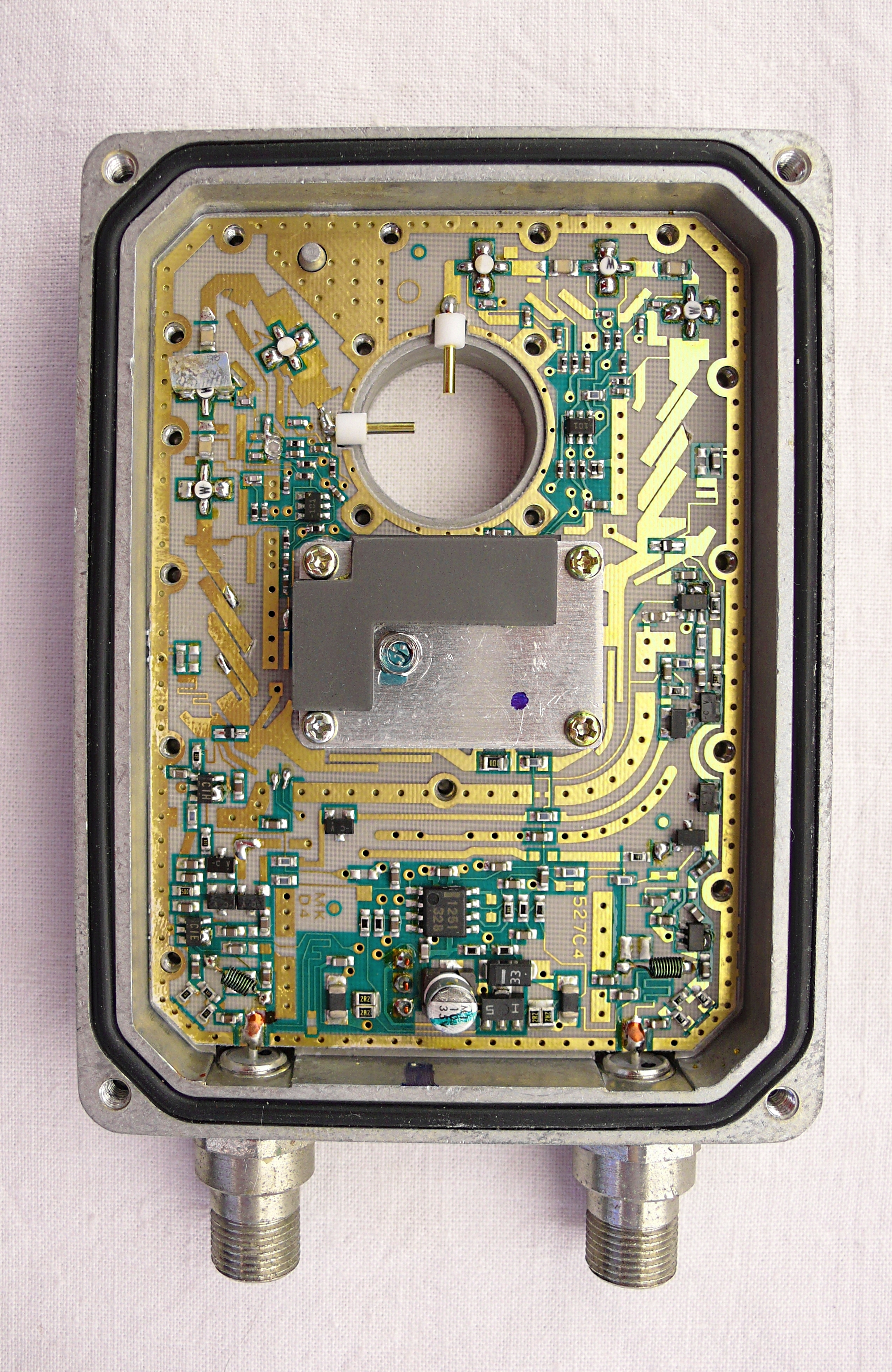
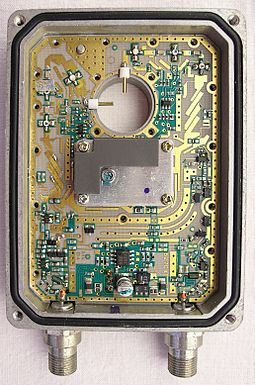 Figure 1. A circuit featuring many of the filter structures described in this article. The operating frequency of the filters is around 11 gigahertz (GHz). This circuit is described in the box below.
Low-noise block converter The circuit depicted in figure 1 is a low-noise block converter and is intended to be attached to a satellite television receiving dish antenna. It is called a block converter because it converts a large number of satellite channels as a block with no attempt to tune to a particular channel. Even though the transmission has travelled 22,000 miles from the satellite orbit, there is a problem getting the signal the last few feet from the dish to the point where it will be used inside the property. The difficulty is that the signal is brought inside the property by a cable (called a downlead) and the high satellite signal frequencies are greatly attenuated when in a cable rather than free space. The purpose of the block converter is to convert the satellite signal to a much lower frequency band that can be handled by the downlead and the user's set-top box. Frequencies depend on satellite system and geographical region, but this particular device converts a block of frequencies in the band 10.7 GHz to 11.8 GHz. The output going to the downlead is in the band 950 MHz to 1950 MHz. The two F connectors at the bottom of the device are for connection to downleads. Two are provided on this particular model (block converters can have any number of outputs from one upwards) so that two televisions or a television and VCR can be tuned to two different channels at the same time. The receiving horn would normally be fitted to the circular hole in the centre of the board, the two probes protruding into this space are for receiving horizontally and vertically polarized signals respectively and the device can be switched between these two. Many filter structures can be seen in the circuit: there are two examples of band-pass parallel-coupled lines filters which are there to restrict the incoming signal to the band of interest. The relatively large width of the resonators (compare to the microstrip example below) reflect the wide bandwidth the filter is required to pass. There are also numerous examples of stub filters supplying DC bias to transistors and other devices, the filter being required to prevent the signal from travelling towards the power source. The rows of holes in some tracks, called via fences, are not filtering structures but form part of the enclosure.[1][2][3] A distributed element filter is an electronic filter in which capacitance, inductance and resistance (the elements of the circuit) are not localised in discrete capacitors, inductors and resistors as they are in conventional filters. Its purpose is to allow a range of signal frequencies to pass, but to block others. Conventional filters are constructed from inductors and capacitors, and the circuits so built are described by the lumped element model, which considers each element to be "lumped together" at one place. That model is conceptually simple, but it becomes increasingly unreliable as the frequency of the signal increases, or equivalently as the wavelength decreases. The distributed element model applies at all frequencies, and is used in transmission line theory; many distributed element components are made of short lengths of transmission line. In the distributed view of circuits, the elements are distributed along the length of conductors and are inextricably mixed together. The filter design is usually concerned only with inductance and capacitance, but because of this mixing of elements they cannot be treated as separate "lumped" capacitors and inductors. There is no precise frequency above which distributed element filters must be used but they are especially associated with the microwave band (wavelength less than one metre).
Distributed element filters are used in many of the same applications as lumped element filters, such as selectivity of radio channel, bandlimiting of noise and multiplexing of many signals into one channel. Distributed element filters may be constructed to have any of the bandforms possible with lumped elements (low-pass, band-pass, etc.) with the exception of high-pass, which is usually only approximated. All filter classes used in lumped element designs (Butterworth, Chebyshev, etc.) can be implemented using a distributed element approach.
There are many component forms used to construct distributed element filters, but all have the common property of causing a discontinuity on the transmission line. These discontinuities present a reactive impedance to a wavefront travelling down the line, and these reactances can be chosen by design to serve as approximations for lumped inductors, capacitors or resonators, as required by the filter.[4]
The development of distributed element filters was spurred on by the military need for radar and electronic counter measures during World War II. Lumped element analogue filters had long before been developed but these new military systems operated at microwave frequencies and new filter designs were required. When the war ended, the technology found applications in the microwave links used by telephone companies and other organisations with large fixed-communication networks, such as television broadcasters. Nowadays the technology can be found in several mass-produced consumer items, such as the converters (figure 1 shows an example) used with satellite television dishes.
Contents
General comments
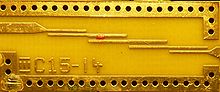 Figure 2. A parallel-coupled lines filter in microstrip construction
- The symbol λ is used to mean the wavelength of the signal being transmitted on the line or a section of line of that electrical length.
Distributed element filters are mostly used at frequencies above the VHF (Very High Frequency) band (30 to 300 MHz). At these frequencies, the physical length of passive components is a significant fraction of the wavelength of the operating frequency, and it becomes difficult to use the conventional lumped element model. The exact point at which distributed element modelling becomes necessary depends on the particular design under consideration. A common rule of thumb is to apply distributed element modelling when component dimensions are larger than 0.1λ. The increasing miniaturisation of electronics has meant that circuit designs are becoming ever smaller compared to λ. The frequencies beyond which a distributed element approach to filter design becomes necessary are becoming ever higher as a result of these advances. On the other hand, antenna structure dimensions are usually comparable to λ in all frequency bands and require the distributed element model.[5]
The most noticeable difference in behaviour between a distributed element filter and its lumped-element approximation is that the former will have multiple passband replicas of the lumped-element prototype passband, because transmission line transfer characteristics repeat at harmonic intervals. These spurious passbands are undesirable in most cases.[6]
For clarity of presentation, the diagrams in this article are drawn with the components implemented in stripline format. This does not imply an industry preference, although planar formats (that is, formats where conductors consist of flat strips) are popular because they can be implemented using established printed circuit board manufacturing techniques. The structures shown can also be implemented using microstrip or buried stripline techniques (with suitable adjustments to dimensions) and can be adapted to coaxial cables, twin leads and waveguides, although some structures are more suitable for some implementations than others. The open wire implementations, for instance, of a number of structures are shown in the second column of figure 3 and open wire equivalents can be found for most other stripline structures. Planar transmission lines are also used in integrated circuit designs.[7]
History
Development of distributed element filters began in the years before World War II. A major paper on the subject was published by Mason and Sykes in 1937.[8] Mason had filed a patent[9] much earlier, in 1927, and that patent may contain the first published design which moves away from a lumped element analysis.[10] Mason and Sykes' work was focused on the formats of coaxial cable and balanced pairs of wires – the planar technologies were not yet in use. Much development was carried out during the war years driven by the filtering needs of radar and electronic counter-measures. A good deal of this was at the MIT Radiation Laboratory,[11] but other laboratories in the US and the UK were also involved.[12][13]
Some important advances in network theory were needed before filters could be advanced beyond wartime designs. One of these was the commensurate line theory of Paul Richards.[14] Commensurate lines are networks in which all the elements are the same length (or in some cases multiples of the unit length), although they may differ in other dimensions to give different characteristic impedances. Richards' transformation allows a lumped element design to be taken "as is" and transformed directly into a distributed element design using a very simple transform equation.[15]
The difficulty with Richards' transformation from the point of view of building practical filters was that the resulting distributed element design invariably included series connected elements. This was not possible to implement in planar technologies and was often inconvenient in other technologies. This problem was solved by K. Kuroda who used impedance transformers to eliminate the series elements. He published a set of transformations known as Kuroda's identities in 1955, but his work was written in Japanese and it was several years before his ideas were incorporated into the English-language literature.[16]
Following the war, one important research avenue was trying to increase the design bandwidth of wide-band filters. The approach used at the time (and still in use today) was to start with a lumped element prototype filter and through various transformations arrive at the desired filter in a distributed element form. This approach appeared to be stuck at a minimum Q of five (see Band-pass filters below for an explanation of Q). In 1957, Leo Young at Stanford Research Institute published a method for designing filters which started with a distributed element prototype.[17] This prototype was based on quarter wave impedance transformers and was able to produce designs with bandwidths up to an octave, corresponding to a Q of about 1.3. Some of Young's procedures in that paper were empirical, but later,[18] exact solutions were published. Young's paper specifically addresses directly coupled cavity resonators, but the procedure can equally be applied to other directly coupled resonator types, such as those found in modern planar technologies and illustrated in this article. The capacitive gap filter (figure 8) and the parallel-coupled lines filter (figure 9) are examples of directly coupled resonators.[15]
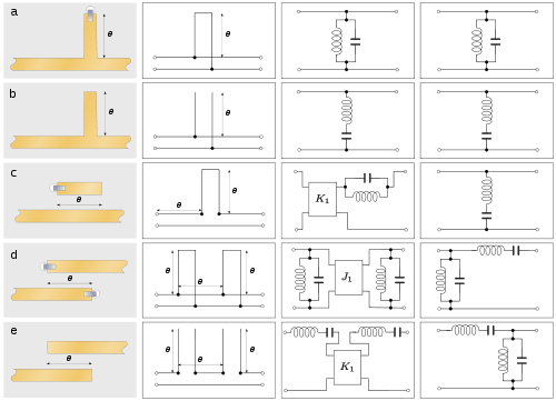 Figure 3. Some simple planar filter structures are shown in the first column. The second column shows the open-wire equivalent circuit for these structures. The third column is a semi-lumped element approximation where the elements marked K or J are impedance or admittance transformers respectively. The fourth column shows a lumped-element approximation making the further assumption that the impedance transformers are λ/4 transformers. (a) A short-circuit stub in parallel with the main line. (b) An open-circuit stub in parallel with the main line. (c) A short-circuit line coupled to the main line. (d) Coupled short-circuited lines. (e) Coupled open-circuited lines.
 represents a strap through the board making connection with the ground plane underneath.
The introduction of printed planar technologies greatly simplified the manufacture of many microwave components including filters, and microwave integrated circuits then became possible. It is not known when planar transmission lines originated, but experiments using them were recorded as early as in 1936.[19] The inventor of printed stripline, however, is known; this was Robert M. Barrett who published the idea in 1951.[20] This caught on rapidly, and Barrett's stripline soon had fierce commercial competition from rival planar formats, especially triplate and microstrip. The generic term stripline in modern usage usually refers to the form then known as triplate.[21]
Early stripline directly-coupled-resonator filters were end-coupled, but the length was reduced and the compactness successively increased with the introduction of parallel-coupled line filters,[22] interdigital filters,[23] and comb-line filters.[24] Much of this work was published by the group at Stanford led by George Matthaei, and also including Leo Young mentioned above, in a landmark book which still today serves as a reference for circuit designers.[25][26] The hairpin filter was first described in 1972.[27][28] By the 1970s, most of the filter topologies in common use today had been described.[29] More recent research has concentrated on new or variant mathematical classes of the filters, such as pseudo-elliptic, while still using the same basic topologies, or with alternative implementation technologies such as suspended stripline and finline.[30]
The initial non-military application of distributed element filters was in the microwave links used by telecommunications companies to provide the backbone of their networks. These links were also used by other industries with large, fixed networks, notably television broadcasters.[31] Such applications were part of large capital investment programs. However, mass-production manufacturing made the technology cheap enough to incorporate in domestic satellite television systems.[32] An emerging application is in superconducting filters for use in the cellular base stations operated by mobile phone companies.[33]
Basic components
The simplest structure that can be implemented is a step in the characteristic impedance of the line, which introduces a discontinuity in the transmission characteristics. This is done in planar technologies by a change in the width of the transmission line. Figure 4(a) shows a step up in impedance (narrower lines have higher impedance). A step down in impedance would be the mirror image of figure 4(a). The discontinuity can be represented approximately as a series inductor, or more exactly, as a low-pass T circuit as shown in figure 4(a).[34] Multiple discontinuities are often coupled together with impedance transformers to produce a filter of higher order. These impedance transformers can be just a short (often λ/4) length of transmission line. These composite structures can implement any of the filter families (Butterworth, Chebyshev, etc.) by approximating the rational function of the corresponding lumped element filter. This correspondence is not exact since distributed element circuits cannot be rational and is the root reason for the divergence of lumped element and distributed element behaviour. Impedance transformers are also used in hybrid mixtures of lumped and distributed element filters (the so-called semi-lumped structures).[35]
Another very common component of distributed element filters is the stub. Over a narrow range of frequencies, a stub can be used as a capacitor or an inductor (its impedance is determined by its length) but over a wide band it behaves as a resonator. Short-circuit, nominally quarter-wavelength stubs (figure 3(a)) behave as shunt LC antiresonators, and an open-circuit nominally quarter-wavelength stub (figure 3(b)) behaves as a series LC resonator. Stubs can also be used in conjunction with impedance transformers to build more complex filters and, as would be expected from their resonant nature, are most useful in band-pass applications.[38] While open-circuit stubs are easier to manufacture in planar technologies, they have the drawback that the termination deviates significantly from an ideal open circuit (see figure 4(b)), often leading to a preference for short-circuit stubs (one can always be used in place of the other by adding or subtracting λ/4 to or from the length).[34]
A helical resonator is similar to a stub, in that it requires a distributed element model to represent it, but is actually built using lumped elements. They are built in a non-planar format and consist of a coil of wire, on a former and core, and connected only at one end. The device is usually in a shielded can with a hole in the top for adjusting the core. It will often look physically very similar to the lumped LC resonators used for a similar purpose. They are most useful in the upper VHF and lower UHF bands whereas stubs are more often applied in the higher UHF and SHF bands.[39]
Coupled lines (figures 3(c-e)) can also be used as filter elements; like stubs, they can act as resonators and likewise be terminated short-circuit or open-circuit. Coupled lines tend to be preferred in planar technologies, where they are easy to implement, whereas stubs tend to be preferred elsewhere. Implementing a true open circuit in planar technology is not feasible because of the dielectric effect of the substrate which will always ensure that the equivalent circuit contains a shunt capacitance. Despite this, open circuits are often used in planar formats in preference to short circuits because they are easier to implement. Numerous element types can be classified as coupled lines and a selection of the more common ones is shown in the figures.[40]
Some common structures are shown in figures 3 and 4, along with their lumped-element counterparts. These lumped-element approximations are not to be taken as equivalent circuits but rather as a guide to the behaviour of the distributed elements over a certain frequency range. Figures 3(a) and 3(b) show a short-circuit and open-circuit stub, respectively. When the stub length is λ/4, these behave, respectively, as anti-resonators and resonators and are therefore useful, respectively, as elements in band-pass and band-stop filters. Figure 3(c) shows a short-circuited line coupled to the main line. This also behaves as a resonator, but is commonly used in low-pass filter applications with the resonant frequency well outside the band of interest. Figures 3(d) and 3(e) show coupled line structures which are both useful in band-pass filters. The structures of figures 3(c) and 3(e) have equivalent circuits involving stubs placed in series with the line. Such a topology is straightforward to implement in open-wire circuits but not with a planar technology. These two structures are therefore useful for implementing an equivalent series element.[41]
Low-pass filters
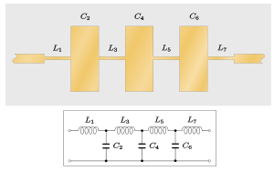 Figure 5. Stepped-impedance low-pass filter formed from alternate high and low impedance sections of line
A low-pass filter can be implemented quite directly from a ladder topology lumped-element prototype with the stepped impedance filter shown in figure 5. The filter consists of alternating sections of high-impedance and low-impedance lines which correspond to the series inductors and shunt capacitors in the lumped-element implementation. Low-pass filters are commonly used to feed direct current (DC) bias to active components. Filters intended for this application are sometimes referred to as chokes. In such cases, each element of the filter is λ/4 in length (where λ is the wavelength of the main-line signal to be blocked from transmission into the DC source) and the high-impedance sections of the line are made as narrow as the manufacturing technology will allow in order to maximise the inductance.[42] Additional sections may be added as required for the performance of the filter just as they would for the lumped-element counterpart. As well as the planar form shown, this structure is particularly well suited for coaxial implementations with alternating discs of metal and insulator being threaded on to the central conductor.[43][44][45]
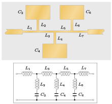 Figure 6. Another form of stepped-impedance low-pass filter incorporating shunt resonators
A more complex example of stepped impedance design is presented in figure 6. Again, narrow lines are used to implement inductors and wide lines correspond to capacitors, but in this case, the lumped-element counterpart has resonators connected in shunt across the main line. This topology can be used to design elliptical filters or Chebyshev filters with poles of attenuation in the stopband. However, calculating component values for these structures is an involved process and has led to designers often choosing to implement them as m-derived filters instead, which perform well and are much easier to calculate. The purpose of incorporating resonators is to improve the stopband rejection. However, beyond the resonant frequency of the highest frequency resonator, the stopband rejection starts to deteriorate as the resonators are moving towards open-circuit. For this reason, filters built to this design often have an additional single stepped-impedance capacitor as the final element of the filter.[46] This also ensures good rejection at high frequency.[47][48][49]
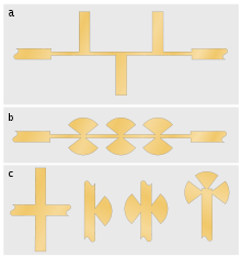 Figure 7. Low-pass filters constructed from stubs. (a) Standard stubs on alternating sides of main line λ/4 apart. (b) Similar construction using butterfly stubs. (c) Various forms of stubs, respectively, doubled stubs in parallel, radial stub, butterfly stub (paralleled radial stubs), clover-leaf stub (triple paralleled radial stubs).
Another common low-pass design technique is to implement the shunt capacitors as stubs with the resonant frequency set above the operating frequency so that the stub impedance is capacitive in the passband. This implementation has a lumped-element counterpart of a general form similar to the filter of figure 6. Where space allows, the stubs may be set on alternate sides of the main line as shown in figure 7(a). The purpose of this is to prevent coupling between adjacent stubs which detracts from the filter performance by altering the frequency response. However, a structure with all the stubs on the same side is still a valid design. If the stub is required to be a very low impedance line, the stub may be inconveniently wide. In these cases, a possible solution is to connect two narrower stubs in parallel. That is, each stub position has a stub on both sides of the line. A drawback of this topology is that additional transverse resonant modes are possible along the λ/2 length of line formed by the two stubs together. For a choke design, the requirement is simply to make the capacitance as large as possible, for which the maximum stub width of λ/4 may be used with stubs in parallel on both sides of the main line. The resulting filter looks rather similar to the stepped impedance filter of figure 5, but has been designed on completely different principles.[42] A difficulty with using stubs this wide is that the point at which they are connected to the main line is ill defined. A stub that is narrow in comparison to λ can be taken as being connected on its centre-line and calculations based on that assumption will accurately predict filter response. For a wide stub, however, calculations that assume the side branch is connected at a definite point on the main line leads to inaccuracies as this is no longer a good model of the transmission pattern. One solution to this difficulty is to use radial stubs instead of linear stubs. A pair of radial stubs in parallel (one on either side of the main line) is called a butterfly stub (see figure 7(b)). A group of three radial stubs in parallel, which can be achieved at the end of a line, is called a clover-leaf stub.[50][51]
Band-pass filters
A band-pass filter can be constructed using any elements that can resonate. Filters using stubs can clearly be made band-pass; numerous other structures are possible and some are presented below.
An important parameter when discussing band-pass filters is the fractional bandwidth. This is defined as the ratio of the bandwidth to the geometric centre frequency. The inverse of this quantity is called the Q-factor, Q. If ω1 and ω2 are the frequencies of the passband edges, then:[52]
- bandwidth
 ,
, - geometric centre frequency
 and
and 
Capacitive gap filter
 Figure 8. Capacitive gap stripline filter
The capacitive gap structure consists of sections of line about λ/2 in length which act as resonators and are coupled "end-on" by gaps in the transmission line. It is particularly suitable for planar formats, is easily implemented with printed circuit technology and has the advantage of taking up no more space than a plain transmission line would. The limitation of this topology is that performance (particularly insertion loss) deteriorates with increasing fractional bandwidth, and acceptable results are not obtained with a Q less than about 5. A further difficulty with producing low-Q designs is that the gap width is required to be smaller for wider fractional bandwidths. The minimum width of gaps, like the minimum width of tracks, is limited by the resolution of the printing technology.[45][53]
Parallel-coupled lines filter
 Figure 9. Stripline parallel-coupled lines filter. This filter is commonly printed at an angle as shown to minimize the board space taken up, although this is not an essential feature of the design. It is also common for the end element or the overlapping halves of the two end elements to be a narrower width for matching purposes (not shown in this diagram, see Figure 1).
Parallel-coupled lines is another popular topology for printed boards, for which open-circuit lines are the simplest to implement since the manufacturing consists of nothing more than the printed track. The design consists of a row of parallel λ/2 resonators, but coupling over only λ/4 to each of the neighbouring resonators, so forming a staggered line as shown in figure 9. Wider fractional bandwidths are possible with this filter than with the capacitive gap filter, but a similar problem arises on printed boards as dielectric loss reduces the Q. Lower-Q lines require tighter coupling and smaller gaps between them which is limited by the accuracy of the printing process. One solution to this problem is to print the track on multiple layers with adjacent lines overlapping but not in contact because they are on different layers. In this way, the lines can be coupled across their width, which results in much stronger coupling than when they are edge-to-edge, and a larger gap becomes possible for the same performance.[54] For other (non-printed) technologies, short-circuit lines may be preferred since the short-circuit provides a mechanical attachment point for the line and Q-reducing dielectric insulators are not required for mechanical support. Other than for mechanical and assembly reasons, there is little preference for open-circuit over short-circuit coupled lines. Both structures can realize the same range of filter implementations with the same electrical performance. Both types of parallel-coupled filters, in theory, do not have spurious passbands at twice the centre frequency as seen in many other filter topologies (e.g. stubs). However, suppression of this spurious passband requires perfect tuning of the coupled lines which is not realized in practice, so there is inevitably some residual spurious passband at this frequency.[45][55][56]
 Figure 10. Stripline hairpin filter
The hairpin filter is another structure that uses parallel-coupled lines. In this case, each pair of parallel-coupled lines is connected to the next pair by a short link. The "U" shapes so formed give rise to the name hairpin filter. In some designs the link can be longer, giving a wide hairpin with λ/4 impedance transformer action between sections.[57][58] The angled bends seen in figure 10 are common to stripline designs and represent a compromise between a sharp right angle, which produces a large discontinuity, and a smooth bend, which takes up more board area which can be severely limited in some products. Such bends are often seen in long stubs where they could not otherwise be fitted into the space available. The lumped-element equivalent circuit of this kind of discontinuity is similar to a stepped-impedance discontinuity.[37] Examples of such stubs can be seen on the bias inputs to several components in the photograph at the top of the article.[45][59]
Interdigital filter
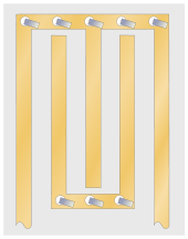 Figure 11. Stripline interdigital filter
Interdigital filters are another form of coupled-line filter. Each section of line is about λ/4 in length and is terminated in a short-circuit at one end only, the other end being left open-circuit. The end which is short-circuited alternates on each line section. This topology is straightforward to implement in planar technologies, but also particularly lends itself to a mechanical assembly of lines fixed inside a metal case. The lines can be either circular rods or rectangular bars, and interfacing to a coaxial format line is easy. As with the parallel-coupled line filter, the advantage of a mechanical arrangement that does not require insulators for support is that dielectric losses are eliminated. The spacing requirement between lines is not as stringent as in the parallel line structure; as such, higher fractional bandwidths can be achieved, and Q values as low as 1.4 are possible.[60][61]
The comb-line filter is similar to the interdigital filter in that it lends itself to mechanical assembly in a metal case without dielectric support. In the case of the comb-line, all the lines are short-circuited at the same end rather than alternate ends. The other ends are terminated in capacitors to ground, and the design is consequently classified as semi-lumped. The chief advantage of this design is that the upper stopband can be made very wide, that is, free of spurious passbands at all frequencies of interest.[62]
Stub band-pass filters
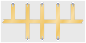 Figure 12. Stripline stub filter composed of λ/4 short-circuit stubs
As mentioned above, stubs lend themselves to band-pass designs. General forms of these are similar to stub low-pass filters except that the main line is no longer a narrow high impedance line. Designers have many different topologies of stub filters to choose from, some of which produce identical responses. An example stub filter is shown in figure 12; it consists of a row of λ/4 short-circuit stubs coupled together by λ/4 impedance transformers. The stubs in the body of the filter are double paralleled stubs while the stubs on the end sections are only singles, an arrangement that has impedance matching advantages. The impedance transformers have the effect of transforming the row of shunt anti-resonators into a ladder of series resonators and shunt anti-resonators. A filter with similar properties can be constructed with λ/4 open-circuit stubs placed in series with the line and coupled together with λ/4 impedance transformers, although this structure is not possible in planar technologies.[63]
 Figure 13. Konishi's 60° butterfly stub
Yet another structure available is λ/2 open-circuit stubs across the line coupled with λ/4 impedance transformers. This topology has both low-pass and band-pass characteristics. Because it will pass DC, it is possible to transmit biasing voltages to active components without the need for blocking capacitors. Also, since short-circuit links are not required, no assembly operations other than the board printing are required when implemented as stripline. The disadvantages are (i) the filter will take up more board real estate than the corresponding λ/4 stub filter, since the stubs are all twice as long; (ii) the first spurious passband is at 2ω0, as opposed to 3ω0 for the λ/4 stub filter.[64]
Konishi describes a wideband 12 GHz band-pass filter, which uses 60° butterfly stubs and also has a low-pass response (short-circuit stubs are required to prevent such a response). As is often the case with distributed element filters, the bandform into which the filter is classified largely depends on which bands are desired and which are considered to be spurious.[65]
High-pass filters
Genuine high-pass filters are difficult, if not impossible, to implement with distributed elements. The usual design approach is to start with a band-pass design, but make the upper stopband occur at a frequency that is so high as to be of no interest. Such filters are described as pseudo-high-pass and the upper stopband is described as a vestigial stopband. Even structures that seem to have an "obvious" high-pass topology, such as the capacitive gap filter of figure 8, turn out to be band-pass when their behaviour for very short wavelengths is considered.[66]
See also
References
- ^ Bahl, pp.290–293.
- ^ Benoit, pp.44–51.
- ^ Lundström, pp.80–82
- ^ Connor, pp.13–14.
- ^ Golio, pp.1.2–1.3,4.4–4.5.
- ^ Matthaei et al., pp.17–18.
- ^ Rogers et al., p.129.
- ^ Mason and Sykes, 1937.
- ^ Mason, Warren P., "Wave filter", U.S. Patent 1,781,469, filed: 25 June 1927, issued: 11 November 1930.
- ^ Fagen and Millman, p.108.
- ^ Ragan, 1965.
- ^ Makimoto and Yamashita, p.2.
- ^ Levy and Cohn, p.1055.
- ^ Richards, 1948.
- ^ a b Levy and Cohn, p.1056.
- ^ Levy and Cohn, p.1057.
- ^ Young, 1963.
- ^ Levy, 1967.
- ^ Aksun, p.142.
- ^ Barrett and Barnes, 1951,
Barrett, 1952,
Niehenke et al., p.846. - ^ Sarkar, pp.556–559.
- ^ Cohn, 1958.
- ^ Matthaei, 1962.
- ^ Matthaei, 1963.
- ^ Matthaei et al., 1964.
- ^ Levy and Cohn, pp.1057–1059.
- ^ Cristal and Frankel, 1972.
- ^ Levy and Cohn, p.1063.
- ^ Niehenke et al., p.847.
- ^ Levy and Cohn, p.1065.
- ^ Huurdeman, pp.369–371.
- ^ Benoit, p.34.
- ^ Ford and Saunders, pp.157–159.
- ^ a b c d Bhat and Koul, p.498.
- ^ Matthaei et al., pp.144–149, 203–207.
- ^ Bhat and Koul, p.539.
- ^ a b c Bhat and Koul, p.499.
- ^ Matthaei et al., pp.203–207.
- ^ Carr, pp.63–64.
- ^ Matthaei et al., pp.217–218.
- ^ Matthaei et al., pp.217–229.
- ^ a b Kneppo, pp.213–214.
- ^ Matthaei et al., pp.373–374.
- ^ Lee, pp.789–790.
- ^ a b c d Sevgi, p.252.
- ^ Hong and Lancaster, p.217.
- ^ Matthaei et al., pp.373–380.
- ^ Lee, pp.792–794.
- ^ Kneppo, p.212.
- ^ Lee, pp.790–792.
- ^ Kneppo, pp.212–213.
- ^ Farago, p.69.
- ^ Matthaei et al., pp.422, 440–450.
- ^ Matthaei et al., pp.585–595.
- ^ Matthaei et al., pp.422, 472–477.
- ^ Kneppo, pp.216–221.
- ^ Hong and Lancaster, pp.130–132.
- ^ Jarry and Beneat, p.15.
- ^ Paolo, pp.113–116.
- ^ Matthaei et al., pp.424, 614–632.
- ^ Hong and Lancaster, p.140.
- ^ Matthaei et al., pp.424, 497–518.
- ^ Matthaei et al., pp.595–605.
- ^ Matthaei et al., pp.605–614.
- ^ Konishi, pp.80–82.
- ^ Matthaei et al., p.541.
Bibliography
- Bahl, I. J. Lumped Elements for RF and Microwave Circuits, Artech House, 2003 ISBN 1-58053-309-4.
- Barrett, R. M. and Barnes, M. H. "Microwave printed circuits", Radio Telev., vol.46, p.16, September 1951.
- Barrett, R. M. "Etched sheets serve as microwave components", Electronics, vol.25, pp.114–118, June 1952.
- Benoit, Hervé Satellite Television: Techniques of Analogue and Digital Television, Butterworth-Heinemann, 1999 ISBN 0-340-74108-2.
- Bhat, Bharathi and Koul, Shiban K. Stripline-like Transmission Lines for Microwave Integrated Circuits, New Age International, 1989 ISBN 81-224-0052-3.
- Carr, Joseph J. The Technician's Radio Receiver Handbook, Newnes, 2001 ISBN 0-7506-7319-2
- Cohn, S. B. "Parallel-coupled transmission-line resonator filters", IRE Transactions: Microwave Theory and Techniques, vol.MTT-6, pp.223–231, April 1958.
- Connor, F. R. Wave Transmission, Edward Arnold Ltd., 1972 ISBN 0-7131-3278-7.
- Cristal, E. G. and Frankel, S. "Hairpin line/half-wave parallel-coupled-line filters", IEEE Transactions: Microwave Theory and Techniques, vol.MTT-20, pp.719–728, November 1972.
- Fagen, M. D. and Millman, S. A History of Engineering and Science in the Bell System: Volume 5: Communications Sciences (1925–1980), AT&T Bell Laboratories, 1984.
- Farago, P. S. An Introduction to Linear Network Analysis, English Universities Press, 1961.
- Ford, Peter John and Saunders, G. A. The Rise of the Superconductors, CRC Press, 2005 ISBN 0-7484-0772-3.
- Golio, John Michael The RF and Microwave Handbook, CRC Press, 2001 ISBN 0-8493-8592-X.
- Hong, Jia-Sheng and Lancaster, M. J. Microstrip Filters for RF/Microwave Applications, John Wiley and Sons, 2001 ISBN 0-471-38877-7.
- Huurdeman, Anton A. The Worldwide History of Telecommunications, Wiley-IEEE, 2003 ISBN 0-471-20505-2.
- Jarry, Pierre and Beneat, Jacques Design and Realizations of Miniaturized Fractal Microwave and RF Filters, John Wiley and Sons, 2009 ISBN 0-470-48781-X.
- Kneppo, Ivan Microwave Integrated Circuits, Springer, 1994 ISBN 0-412-54700-7.
- Konishi, Yoshihiro Microwave Integrated Circuits, CRC Press, 1991 ISBN 0-8247-8199-6.
- Lee, Thomas H. Planar Microwave Engineering: A Practical Guide to Theory, Measurement, and Circuits, Cambridge University Press, 2004 ISBN 0-521-83526-7.
- Levy, R. "Theory of direct coupled-cavity filters", IEEE Transactions: Microwave Theory and Techniques, vol.MTT-15, pp.340–348, June 1967.
- Levy, R. Cohn, S.B., "A History of microwave filter research, design, and development", IEEE Transactions: Microwave Theory and Techniques, pp.1055–1067, vol.32, issue 9, 1984.
- Lundström, Lars-Ingemar Understanding Digital Television, Elsevier, 2006 ISBN 0-240-80906-8.
- Makimoto, Mitsuo and Yamashita, Sadahiko "Microwave resonators and filters for wireless communication: theory, design, and application", Springer, 2001 ISBN 3-540-67535-3.
- Mason, W. P. and Sykes, R. A. "The use of coaxial and balanced transmission lines in filters and wide band transformers for high radio frequencies", Bell Syst. Tech. J., vol.16, pp.275–302, 1937.
- Matthaei, G. L. "Interdigital band-pass filters", IRE Transactions: Microwave Theory and Techniques, vol.MTT-10, pp.479–491, November 1962.
- Matthaei, G. L. "Comb-line band-pass filters of narrow or moderate bandwidth", Microwave Journal, vol.6, pp.82–91, August 1963.
- Matthaei, George L.; Young, Leo and Jones, E. M. T. Microwave Filters, Impedance-Matching Networks, and Coupling Structures McGraw-Hill 1964 (1980 edition is ISBN 0-89006-099-1).
- Niehenke, E. C.; Pucel, R. A. and Bahl, I. J. "Microwave and millimeter-wave integrated circuits", IEEE Transactions: Microwave Theory and Techniques, 'vol.50, Iss.3 March 2002, pp.846–857.
- Di Paolo, Franco Networks and Devices using Planar Transmission Lines, CRC Press, 2000 ISBN 0-8493-1835-1.
- Ragan, G. L. (ed.) Microwave transmission circuits, Massachusetts Institute of Technology Radiation Laboratory, Dover Publications, 1965.
- Richards, P. I. "Resistor-transmission-line circuits", Proceedings of the IRE, vol.36, pp.217–220, Feb. 1948.
- Rogers, John W. M. and Plett, Calvin Radio Frequency Integrated Circuit Design, Artech House, 2003 ISBN 1-58053-502-X.
- Sarkar, Tapan K. History of Wireless, John Wiley and Sons, 2006 ISBN 0-471-71814-9.
- Sevgi, Levent Complex Electromagnetic Problems and Numerical Simulation Approaches, Wiley-IEEE, 2003 ISBN 0-471-43062-5.
- Young, L. "Direct-coupled cavity filters for wide and narrow bandwidths" IEEE Transactions: Microwave Theory and Techniques, vol.MTT-11, pp.162–178, May 1963.
Categories:- Distributed element circuits
- Microwave technology


Wikimedia Foundation. 2010.