Heritability

Heritability is the proportion of phenotypic variation in a population that is due to genetic variation between individuals. Phenotypic variation among individuals may be due to genetic, environmental factors, and/or random chance^[1]. Heritability analyzes the relative contributions of differences in genetic and non-genetic factors to the total phenotypic variance in a population. It is measured by estimating the relative contributions of genetic and non-genetic differences to the total phenotypic variation in a population. Heritability is an important concept in quantitative genetics, particularly in selective breeding and behaviour genetics (for instance twin studies), but is less widely used in population genetics.

Heritability measures the fraction of phenotype variability that can be attributed to genetic variation. This is not the same as saying that this fraction of an individual phenotype is caused by genetics. In addition, heritability can change without any genetic change occurring. For example, if both genes and environment have the potential to influence intelligence, but if a given sample of individuals shows very little genetic variation and a great deal of environmental variation, then the contribution of genetic variability to phenotype variability in that sample will be lower than if the sample showed greater genetic variability. Because of this it can be seen that heritability is specific to a particular population in a particular environment.

The extent of dependence of phenotype on environment can also be function of the genes involved. Genes may canalize a phenotype, making its expression almost inevitable in all occurring environments. Individuals with the same genotype can exhibit different phenotypes through a mechanism called phenotypic plasticity, which makes heritability difficult to measure in some cases. Recent insights in molecular biology have identified changes in transcriptional activity of individual genes associated with environmental changes. However, there are a large number of genes whose transcription is not affected by the environment.^[2]

Overview

An example of low heritability: a population with genotypes coding for only one hair colour

A crowd with variance in hair colour.

Heritability estimates use statistical analyses to help to identify the causes of differences between individuals. Because heritability is concerned with variance, it is necessarily an account of the differences between individuals in a population. Heritability can be univariate – examining a single traits – or multivariate – examining the genetic and environmental associations between multiple traits at once. This allows a test of the genetic overlap between different phenotypes: for instance hair colour and eye colour. Environment and genetics may also interact, and heritability analyses can test for and examine these interactions (GxE models).

A prerequisite for heritability analyses is that there is some population variation to account for. In practice, all traits vary and almost all traits show some heritability.^[3] For example, in a population with no diversity in hair colour, "heritability" of hair colour would be undefined. In populations with varying values of a trait (such as the hair colours shown below), variance could be due to environment (hair dye for instance) or genetic differences, and heritability could vary from 0-100%.

This last point highlights the fact that heritability cannot take into account the effect of factors which are invariant in the population: Either because they don't exist (an unavailable anti-biotic), or because they are omni-present (perhaps drinking coffee is approaching that level of exposure).

Definition

Any particular phenotype can be modelled as the sum of genetic and environmental effects:^[4]

Phenotype (P) = Genotype (G) + Environment (E).

Likewise the variance in the trait – Var (P) – is the sum of genetic effects as follows:

Var(P) = Var(G) + Var(E) + 2 Cov(G,E).

In a planned experiment Cov(G,E) can be controlled and held at 0. In this case, heritability is defined as:

$H^2 = \frac{Var(G)}{Var(P)}$ .

H² is the broad-sense heritability. This reflects all the genetic contributions to a population's phenotypic variance including additive, dominant, and epistatic (multi-genic interactions), as well as maternal and paternal effects, where individuals are directly affected by their parents' phenotype (such as with milk production in mammals).

These additional terms can be decomposed in some genetic models. 'An important example is capturing only portion of the variance due to additive (allelic) genetic effects. This additive genetic portion is known as Narrow-sense heritability' and is defined as

$h^2 = \frac{Var(A)}{Var(P)}$

An upper case H² is used to denote broad sense, and lower case h² for narrow sense.

Additive variance is important for selection. If a selective pressure such as improving livestock is exerted, the response of the trait is directly related to narrow-sense heritability. The mean of the trait will increase in the next generation as a function of how much the mean of the selected parents differs from the mean of the population from which the selected parents were chosen. The observed response to selection leads to an estimate of the narrow-sense heritability (called realized heritability). This is the principle underlying artificial selection or breeding.

Example

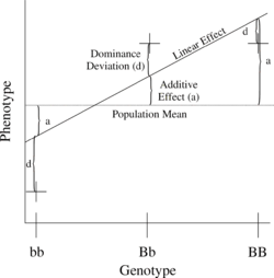Figure 1. Relationship of phenotypic values to additive and dominance effects using a completely dominant locus.

The simplest genetic model involves a single locus with two alleles (b and B) affecting one quantitative phenotype.

The number of B alleles can vary from 0, 1, or 2. For any genotype, B_iB_j, the expected phenotype can then be written as the sum of the overall mean, a linear effect, and a dominance deviation:

P_ij = μ + α_i + α_j + d_ij = Population mean + Additive Effect (a_ij = α_i + α_j) + Dominance Deviation (d_ij).

The additive genetic variance at this locus is the weighted average of the squares of the additive effects:

$Var(A) = f(bb)a^2_{bb}+f(Bb)a^2_{Bb}+f(BB)a^2_{BB},$

where f(bb)a_bb + f(Bb)a_Bb + f(BB)a_BB = 0.

There is a similar relationship for variance of dominance deviations:

$Var(D) = f(bb)d^2_{bb}+f(Bb)d^2_{Bb}+f(BB)d^2_{BB},$

where f(bb)d_bb + f(Bb)d_Bb + f(BB)d_BB = 0.

The linear regression of phenotype on genotype is shown in Figure 1.

Estimating heritability

Since only P can be observed or measured directly, heritability must be estimated from the similarities observed in subjects varying in their level of genetic or environmental similarity. The statistical analyses required to estimate the genetic and environmental components of variance depend on the sample characteristics. Briefly, better estimates are obtained using data from individuals with widely varying levels of genetic relationship - such as twins, siblings, parents and offspring, rather than from more distantly related (and therefore similar) subjects. The standard error for heritability estimates is improved with large sample sizes.

In non-human populations it is often possible to collect information in a controlled way. For example, among farm animals it is easy to arrange for a bull to produce offspring from a large number of cows and to control environments. Such experimental control is impossible when gathering human data, relying on naturally occurring relationships and environments.

Studies of human heritability often utilise adoption study designs, often with identical twins who have been separated early in life and raised in different environments (see for example Fig. 2). Such individuals have identical genotypes and can be used to separate the effects of genotype and environment. A limit of this design is the common prenatal environment and the relatively low numbers of twins reared apart. A second and more common design is the twin study in which the similarity of identical and fraternal twins is used to estimate heritability. entail problems of their own, such as: identical twins are not completely genetically identical. Studies of twins also examine differences between twins and non-twin siblings, for instance to examine phenomena such as intrauterine competition (for example, twin-to-twin transfusion syndrome).

Heritability estimates are always relative to the genetic and environmental factors in the population, and are not absolute measurements of the contribution of genetic and environmental factors to a phenotype. Heritability estimates reflect the amount of variation in genotypic effects compared to variation in environmental effects.

Heritability can be made larger by diversifying the genetic background, e.g., by using only very outbred individuals (which increases Var_G) and/or by minimizing environmental effects (decreasing Var_E). The converse also holds. Due to such effects, different populations of a species might have different heritabilities for the same trait.

In observational studies, or because of evokative effects (where a genome evokes environments by its effect on them), G and E may covary: gene environment correlation. Depending on the methods used to estimate heritability, correlations between genetic factors and shared or non-shared environments may or may not be confounded with heritability.^[5]

Heritability estimates are often misinterpreted if it is not understood that they refer to the proportion of variation between individuals in a population that is influenced by genetic factors. Heritability describes the population, not individuals within that population. For example, It is incorrect to say that since the heritability of a personality trait is about .6, that means that 60% of your personality is inherited from your parents and 40% comes from the environment.

A highly heritable trait (such as eye color) assumes environmental inputs which (though they are invariant in most populations) are required for development: for instance temperatures and atmospheres supporting life, etc.). A more useful distinction than "nature vs. nurture" is "obligate vs. facultative" -- under typical environmental ranges, what traits are more "obligate" (e.g., the nose—everyone has a nose) or more "facultative" (sensitive to environmental variations, such as specific language learned during infancy). Another useful distinction is between traits that are likely to be adaptations (such as the nose) vs. those that are byproducts of adaptations (such the white color of bones), or are due to random variation (non-adaptive variation in, say, nose shape or size).

Estimation methods

There are essentially two schools of thought regarding estimation of heritability.

One school of thought was developed by Sewall Wright at The University of Chicago, and further popularized by C. C. Li (University of Chicago) and J. L. Lush (Iowa State University). It is based on the analysis of correlations and, by extension, regression. Path Analysis was developed by Sewall Wright as a way of estimating heritability.

The second was originally developed by R. A. Fisher and expanded at The University of Edinburgh, Iowa State University, and North Carolina State University, as well as other schools. It is based on the analysis of variance of breeding studies, using the intraclass correlation of relatives. Various methods of estimating components of variance (and, hence, heritability) from ANOVA are used in these analyses.

Regression/correlation methods of estimation

The first school of estimation uses regression and correlation to estimate heritability.

Selection experiments

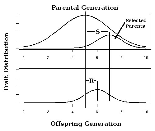
Figure 3. Strength of selection (S) and response to selection (R) in an artificial selection experiment, h²=R/S.

Calculating the strength of selection, S (the difference in mean trait between the population as a whole and the selected parents of the next generation, also called the selection differential^[6]) and response to selection R (the difference in offspring and whole parental generation mean trait) in an artificial selection experiment will allow calculation of realized heritability as the response to selection relative to the strength of selection, h²=R/S as in Fig. 3.

Comparison of close relatives

In the comparison of relatives, we find that in general,

$h^2 = \frac{b}{r} = \frac{t}{r}$ where r can be thought of as the coefficient of relatedness, b is the coefficient of regression and t the coefficient of correlation.

Parent-offspring regression

Figure 4. Sir Francis Galton's (1889) data showing the relationship between offspring height (928 individuals) as a function of mean parent height (205 sets of parents).

Heritability may be estimated by comparing parent and offspring traits (as in Fig. 4). The slope of the line (0.57) approximates the heritability of the trait when offspring values are regressed against the average trait in the parents. If only one parent's value is used then heritability is twice the slope. (note that this is the source of the term "regression", since the offspring values always tend to regress to the mean value for the population, i.e., the slope is always less than one). This regression effect also underlies the DeFries Fulker method for analysing twins selected for one member being affected. ^[7]

Sibling comparison

A basic approach to heritability can be take using full-sib designs: comparing similarity between siblings who share both a biological mother and a father ^[8]. When there is only additive gene action, this sibling phenotypic correlation is an index of familiarity – the sum of half the additive genetic variance plus full effect of the common environment . It thus places an upper-limit on additive heritability of twice the full-sib phenotypic correlation. Half-sib designs compare phenotypic traits of siblings that share one parent with other sibling groups.

Twin studies

Main article: twin study

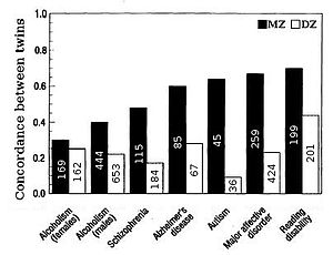Figure 5. Twin concordances for seven psychological traits (sample size shown inside bars).

Heritability for traits in humans is most frequently estimated by comparing resemblances between twins (Fig. 2 & 5). Fraternal (DZ) twins on average share half their genes (see Assortative mating) and so identical (MZ) twins on average are twice as genetically similar as DZ twins. A crude estimate of heritability, then, is approximately twice the difference in correlation between MZ and DZ twins, i.e. Falconer's formula H²=2(r(MZ)-r(DZ)).

The effect of shared environment, c², contributes to similarity between siblings due to the commonality of the environment they are raised in. Shared environment is approximated by the DZ correlation minus half heritability, which is the degree to which DZ twins share the same genes, c²=DZ-1/2h². Unique environmental variance, e², reflects the degree to which identical twins raised together are dissimilar, e²=1-r(MZ).

The methodology of the classical twin study has been criticized, but some of these criticisms do not take into account the methodological innovations and refinements described above.

Extended pedigree design

While often heritability is analysed in single generations: comparing MZ twins raised apart, or comparing the similarity of MZ and DZ twins, considerable power can be gained using more complex relationships. By studying a trait in multi-generational families, the multiple recombinations of genetic and environmental effects can be decomposed using software such as ASReml and heritability estimated ^[9]. This design is especially powerful for untangling confounds such as reverse causality, maternal effects such as the prenatal environment, and confounding of genetic dominance, shared environment, and maternal gene effects ^{[10] [11]}

Analysis of variance methods of estimation

The second set of methods of estimation of heritability involves ANOVA and estimation of variance components.

Basic model

We use the basic discussion of Kempthorne (1957 [1969]). Considering only the most basic of genetic models, we can look at the quantitative contribution of a single locus with genotype G_i as

y_i = μ + g_i + e

where

g_i is the effect of genotype G_i

and e is the environmental effect.

Consider an experiment with a group of sires and their progeny from random dams. Since the progeny get half of their genes from the father and half from their (random) mother, the progeny equation is

$z_i = \mu + \frac{1}{2}g_i + e$

Intraclass correlations

Consider the experiment above. We have two groups of progeny we can compare. The first is comparing the various progeny for an individual sire (called within sire group). The variance will include terms for genetic variance (since they did not all get the same genotype) and environmental variance. This is thought of as an error term.

The second group of progeny are comparisons of means of half sibs with each other (called among sire group). In addition to the error term as in the within sire groups, we have an addition term due to the differences among different means of half sibs. The intraclass correlation is

$corr(z,z') = corr(\mu + \frac{1}{2}g + e, \mu + \frac{1}{2}g + e') = \frac{1}{4}V_g$ ,

since environmental effects are independent of each other.

The ANOVA

In an experiment with n sires and r progeny per sire, we can calculate the following ANOVA, using V_g as the genetic variance and V_e as the environmental variance:

Table 1: ANOVA for Sire experiment

Source	d.f.	Mean Square	Expected Mean Square
Among sire groups	n − 1	S	$\frac{3}{4}V_g + V_e + r({\frac{1}{4}V_g})$
Within sire groups	n(r − 1)	W	$\frac{3}{4}V_g + V_e$

The $\frac{1}{4}V_g$ term is the intraclass correlation among half sibs. We can easily calculate $H^2 = \frac{V_g}{V_g+V_e} = \frac{4(S-W)}{S+(r-1)W}$. The Expected Mean Square is calculated from the relationship of the individuals (progeny within a sire are all half-sibs, for example), and an understanding of intraclass correlations.

Model with additive and dominance terms

For a model with additive and dominance terms, but not others, the equation for a single locus is

y_ij = μ + α_i + α_j + d_ij + e,

where

α_i is the additive effect of the i^th allele, α_j is the additive effect of the j^th allele, d_ij is the dominance deviation for the ij^th genotype, and e is the environment.

Experiments can be run with a similar setup to the one given in Table 1. Using different relationship groups, we can evaluate different intraclass correlations. Using V_a as the additive genetic variance and V_d as the dominance deviation variance, intraclass correlations become linear functions of these parameters. In general,

Intraclass correlation = rV_a + θV_d,

where r and θ are found as

r = P[ alleles drawn at random from the relationship pair are identical by descent], and

θ = P[ genotypes drawn at random from the relationship pair are identical by descent].

Some common relationships and their coefficients are given in Table 2.

Table 2: Coefficients for calculating variance components

Relationship	r	θ
Identical Twins	1	1
Parent-Offspring	$\frac{1}{2}$	0
Half Siblings	$\frac{1}{4}$	0
Full Siblings	$\frac{1}{2}$	$\frac{1}{4}$
First Cousins	$\frac{1}{8}$	0
Double First Cousins	$\frac{1}{4}$	$\frac{1}{16}$

Larger models

When a large, complex pedigree is available for estimating heritability, the most efficient use of the data is in a restricted maximum likelihood (REML) model. The raw data will usually have three or more datapoints for each individual: a code for the sire, a code for the dam and one or several trait values. Different trait values may be for different traits or for different timepoints of measurement.

The currently popular methodology relies on high degrees of certainty over the identities of the sire and dam; it is not common to treat the sire identity probabilistically. This is not usually a problem, since the methodology is rarely applied to wild populations (although it has been used for several wild ungulate and bird populations), and sires are invariably known with a very high degree of certainty in breeding programmes. There are also algorithms that account for uncertain paternity.

The pedigrees can be viewed using programs such as Pedigree Viewer [2], and analysed with programs such as ASReml, VCE [3], WOMBAT [4] or BLUPF90 family's programs [5]

Response to Selection

In selective breeding of plants and animals, the expected response to selection can be estimated by the following equation:^[12]

R = h²S

In this equation, the Response to Selection (R) is defined as the realized average difference between the parent generation and the next generation. The Selection Differential (S) is defined as the average difference between the parent generation and the selected parents.

For example, imagine that a plant breeder is involved in a selective breeding project with the aim of increasing the number of kernels per ear of corn. For the sake of argument, let us assume that the average ear of corn in the parent generation has 100 kernels. Let us also assume that the selected parents produce corn with an average of 120 kernels per ear. If h² equals 0.5, then the next generation will produce corn with an average of 0.5(120-100) = 10 additional kernels per ear. Therefore, the total number of kernels per ear of corn will equal, on average, 110.

Controversies

Some authors like Steven Rose^[13] and Jay Joseph^[14] have dismissed heritability estimates as useless. A 2008 paper in Nature Reviews Genetics stated however: "Despite continuous misunderstandings and controversies over its use and application, heritability remains key to the response to selection in evolutionary biology and agriculture, and to the prediction of disease risk in medicine. Recent reports of substantial heritability for gene expression and new estimation methods using marker data highlight the relevance of heritability in the genomics era."^[15]

See also

• Heredity
• Heritability of IQ

References

Notes

1. ^ Raj A, van Oudenaarden A. 2008. "Nature, nurture, or chance: stochastic gene expression and its consequences." PMID 18957198
2. ^ http://jhered.oxfordjournals.org/content/98/4/382.full
3. ^ E. Turkheimer. (2000). Three laws of behavior genetics and what they mean. Current directions in psychological science, 9, 160-164.
4. ^ Kempthorne (1957)
5. ^ Cattell RB (1960). "The multiple abstract variance analysis equations and solutions: for nature–nurture research on continuous variables". Psychol Rev 67 (6): 353–372. doi:10.1037/h0043487. PMID 13691636. 
6. ^ Kempthorne (1957), page 507; or Falconer (1960), page 191, for example.
7. ^ J. C. DeFries and D. W. Fulker. (1985). Multiple regression analysis of twin data. Behavior Genetics, 15, [1]
8. ^ D. S. Falconer and T. F. C. Mackay. (1996). Introduction to Quantitative Genetics. Journal
9. ^ M. Luciano, G. D. Batty, M. McGilchrist, P. Linksted, B. Fitzpatrick, C. Jackson, A. Pattie, A. F. Dominiczak, A. Morris, B. H. Smith, D. Porteous and I. J. Deary. (2010). Shared genetic aetiology between cognitive ability and cardiovascular disease risk factors: Generation Scotland's Scottish family health study. Intelligence, 38, 304-313
10. ^ W. G. Hill, M. E. Goddard and P. M. Visscher. (2008). Data and theory point to mainly additive genetic variance for complex traits. PLoS Genet, 4, e1000008
11. ^ P. M. Visscher, W. G. Hill and N. R. Wray. (2008). Heritability in the genomics era - concepts and misconceptions. Nature Reviews Genetics, 9, 255-266
12. ^ Plomin, R., DeFries, J. C., & McClearn, G. E. (1990). Behavioral genetics. New York: Freeman.
13. ^ Rose SP (June 2006). "Commentary: heritability estimates--long past their sell-by date". Int J Epidemiol 35 (3): 525–7. doi:10.1093/ije/dyl064. PMID 16645027. 
14. ^ Joseph, J. (2004), The Gene Illusion, Algora. (2003 United Kingdom Edition by PCCS Books) (Chapter 5 contains a critique of the heritability concept)
15. ^ Visscher, P. M.; Hill, W. G.; Wray, N. R. (2008). "Heritability in the genomics era — concepts and misconceptions". Nature Reviews Genetics 9 (4): 255–66. doi:10.1038/nrg2322. PMID 18319743.  edit

Books

• Kempthorne, O (1957 [1969]) An Introduction to Genetic Statistics. John Wiley. Reprinted, 1969 by Iowa State University Press.

Further reading

• Gillespie, G. H. (1997). Population Genetics: A Concise Guide. Johns Hopkins University Press.
• Lynch, M. & Walsh, B. 1997. Genetics and Analysis of Quantitative Traits. Sinauer Associates. ISBN 0-87893-481-2.
• Maher, B. (2008). "Personal genomes: the case of the missing heritability". Nature 456 (7218): 18–21. doi:10.1038/456018a. PMID 18987709.  edit

External links

• Stanford Encyclopedia of Philosophy entry on Heredity and Heritability
• Quantitative Genetics Resources website, including the two volume book by Lynch and Walsh. Free access