Viscoplasticity

Figure 1. Elements used in one-dimensional models of viscoplastic materials.

Viscoplasticity is a theory in continuum mechanics that describes the rate-dependent inelastic behavior of solids. Rate-dependence in this context means that the deformation^{[disambiguation needed ]} of the material depends on the rate at which loads are applied.^[1] The inelastic behavior that is the subject of viscoplasticity is plastic deformation which means that the material undergoes unrecoverable deformations when a load level is reached. Rate-dependent plasticity is important for transient plasticity calculations. The main difference between rate-independent plastic and viscoplastic material models is that the latter exhibit not only permanent deformations after the application of loads but continue to undergo a creep flow as a function of time under the influence of the applied load.

The elastic response of viscoplastic materials can be represented in one-dimension by Hookean spring elements. Rate-dependence can be represented by nonlinear dashpot elements in a manner similar to viscoelasticity. Plasticity can be accounted for by adding sliding frictional elements as shown in Figure 1.^[2] In the figure E is the modulus of elasticity, λ is the viscosity parameter and N is a power-law type parameter that represents non-linear dashpot [σ(dε/dt)= σ = λ(dε/dt)^(1/N)]. The sliding element can have a yield stress (σ_y) that is strain rate dependent, or even constant, as shown in Figure 1c.

Viscoplasticity is usually modeled in three-dimensions using overstress models of the Perzyna or Duvaut-Lions types.^[3] In these models, the stress is allowed to increase beyond the rate-independent yield surface upon application of a load and then allowed to relax back to the yield surface over time. The yield surface is usually assumed not to be rate-dependent in such models. An alternative approach is to add a strain rate dependence to the yield stress and use the techniques of rate independent plasticity to calculate the response of a material^[4]

For metals and alloys, viscoplasticity is the macroscopic behavior caused by a mechanism linked to the movement of dislocations in grains, with superposed effects of inter-crystalline gliding^{[disambiguation needed ]}. The mechanism usually becomes dominant at temperatures greater than approximately one third of the absolute melting temperature. However, certain alloys exhibit viscoplasticity at room temperature (300K). For polymers, wood, and bitumen, the theory of viscoplasticity is required to describe behavior beyond the limit of elasticity or viscoelasticity.

In general, viscoplasticity theories are useful in areas such as

• the calculation of permanent deformations,
• the prediction of the plastic collapse of structures,
• the investigation of stability,
• crash simulations,
• systems exposed to high temperatures such as turbines in engines, e.g. a power plant,
• dynamic problems and systems exposed to high strain rates.

History

Research on plasticity theories started in 1864 with the work of Henri Tresca,^[5] Saint Venant (1870) and Levy^{[disambiguation needed ]} (1871)^[6] on the maximum shear criterion.^[7] An improved plasticity model was presented in 1913 by Von Mises^[8] which is now referred to as the von Mises yield criterion. In viscoplasticity, the development of a mathematical model heads back to 1910 with the representation of primary creep by Andrade's law.^[9] In 1929, Norton^[10] developed a one-dimensional dashpot model which linked the rate of secondary creep to the stress. In 1934, Odqvist^[11] generalized Norton's law to the multi-axial case.

Concepts such as the normality of plastic flow to the yield surface and flow rules for plasticity were introduced by Prandtl (1924)^[12] and Reuss^{[disambiguation needed ]} (1930).^[13] In 1932, Hohenemser and Prager ^[14] proposed the first model for slow viscoplastic flow. This model provided a relation between the deviatoric stress and the strain rate for an incompressible Bingham solid^[15] However, the application of these theories did not begin before 1950, where limit theorems were discovered.

In 1960, the first IUTAM Symposium “Creep in Structures” organized by Hoff^[16] provided a major development in viscoplasticity with the works of Hoff, Rabotnov, Perzyna, Hult, and Lemaitre for the isotropic hardening laws, and those of Kratochvil, Malinini and Khadjinsky, Ponter and Leckie, and Chaboche for the kinematic hardening laws. Perzyna, in 1963, introduced a viscosity coefficient that is temperature and time dependent.^[17] The formulated models were supported by the thermodynamics of irreversible processes and the phenomenological standpoint. The ideas presented in these works have been the basis for most subsequent research into rate-dependent plasticity.

Phenomenology

For a qualitative analysis, several characteristic tests are performed to describe the phenomenology of viscoplastic materials. Some examples of these tests are ^[9]

1. hardening tests at constant stress or strain rate,
2. creep tests at constant force, and
3. stress relaxation at constant elongation.

Strain hardening test

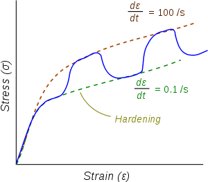Figure 2. Stress-strain response of a viscoplastic material at different strain rates. The dotted lines show the response if the strain-rate is held constant. The blue line shows the response when the strain rate is changed suddenly.

One consequence of yielding is that as plastic deformation proceeds, an increase in stress is required to produce additional strain. This phenomenon is known as Strain/Work hardening.^[18] For a viscoplastic material the hardening curves are not significantly different from those of rate-independent plastic material. Nevertheless, three essential differences can be observed.

1. At the same strain, the higher the rate of strain the higher the stress
2. A change in the rate of strain during the test results in an immediate change in the stress–strain curve.
3. The concept of a plastic yield limit is no longer strictly applicable.

The hypothesis of partitioning the strains by decoupling the elastic and plastic parts is still applicable where the strains are small,^[3] i.e.,

$\boldsymbol{\varepsilon} = \boldsymbol{\varepsilon}_{\mathrm{e}} + \boldsymbol{\varepsilon}_{\mathrm{vp}}$

where $\boldsymbol{\varepsilon}_{\mathrm{e}}$ is the elastic strain and $\boldsymbol{\varepsilon}_{\mathrm{vp}}$ is the viscoplastic strain. To obtain the stress-strain behavior shown in blue in the figure, the material is initially loaded at a strain rate of 0.1/s. The strain rate is then instantaneously raised to 100/s and held constant at that value for some time. At the end of that time period the strain rate is dropped instantaneously back to 0.1/s and the cycle is continued for increasing values of strain. There is clearly a lag between the strain-rate change and the stress response. This lag is modeled quite accurately by overstress models (such as the Perzyna model) but not by models of rate-independent plasticity that have a rate-dependent yield stress.

Creep test

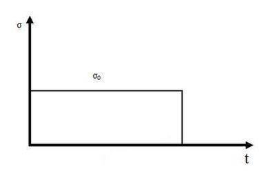
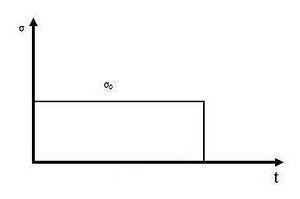Figure 3a. Creep test

Figure 3b. Strain as a function of time in a creep test.

Creep is the tendency of a solid material to slowly move or deform permanently under constant stresses. Creep tests measure the strain response due to a constant stress as shown in Figure 3. The classical creep curve represents the evolution of strain as a function of time in a material subjected to uniaxial stress at a constant temperature. The creep test, for instance, is performed by applying a constant force/stress and analyzing the strain response of the system. In general, as shown in Figure 3b this curve usually shows three phases or periods of behavior^[9]

1. A primary creep stage, also known as transient creep, is the starting stage during which hardening of the material leads to a decrease in the rate of flow which is initially very high. $(0 \le \boldsymbol{\varepsilon} \le \boldsymbol{\varepsilon}_1 )$.
2. The secondary creep stage, also known as the steady state, is where the strain rate is constant. $(\boldsymbol{\varepsilon}_1 \le \boldsymbol{\varepsilon} \le \boldsymbol{\varepsilon}_2)$.
3. A tertiary creep phase in which there is an increase in the strain rate up to the fracture strain. $(\boldsymbol{\varepsilon}_2 \le \boldsymbol{\varepsilon} \le \boldsymbol{\varepsilon}_R)$.

Relaxation test

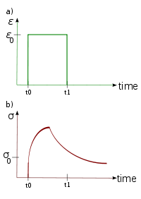Figure 4. a) Applied strain in a relaxation test and b) induced stress as functions of time over a short period for a viscoplastic material.

As shown in Figure 4, the relaxation test^[19] is defined as the stress response due to a constant strain for a period of time. In viscoplastic materials, relaxation tests demonstrate the stress relaxation in uniaxial loading at a constant strain. In fact, these tests characterize the viscosity and can be used to determine the relation which exists between the stress and the rate of viscoplastic strain. The decompositon of strain rate is

$\cfrac{\mathrm{d}\boldsymbol{\varepsilon}}{\mathrm{d}t} = \cfrac{\mathrm{d}\boldsymbol{\varepsilon}_{\mathrm{e}}}{\mathrm{d}t} + \cfrac{\mathrm{d}\boldsymbol{\varepsilon}_{\mathrm{vp}}}{\mathrm{d}t} ~.$

The elastic part of the strain rate is given by

$\cfrac{\mathrm{d}\boldsymbol{\varepsilon}_{\mathrm{e}}}{\mathrm{d}t} = \mathsf{E}^{-1}~\cfrac{\mathrm{d}\boldsymbol{\sigma}}{\mathrm{d}t}$

For the flat region of the strain-time curve, the total strain rate is zero. Hence we have,

$\cfrac{\mathrm{d}\boldsymbol{\varepsilon}_{\mathrm{vp}}}{\mathrm{d}t} = -\mathsf{E}^{-1}~\cfrac{\mathrm{d}\boldsymbol{\sigma}}{\mathrm{d}t}$

Therefore the relaxation curve can be used to determine rate of viscoplastic strain and hence the viscosity of the dashpot in a one-dimensional viscoplastic material model. The residual value that is reached when the stress has plateaued at the end of a relaxation test corresponds to the upper limit of elasticity. For some materials such as rock salt such an upper limit of elasticity occurs at a very small value of stress and relaxation tests can be continued for more than a year without any observable plateau in the stress.

It is important to note that relaxation tests are extremely difficult to perform because maintaining the condition $\cfrac{\mathrm{d}\boldsymbol{\varepsilon}}{\mathrm{d}t} = 0$ in a test requires considerable delicacy.^[20]

Rheological models of viscoplasticity

One-dimensional constitutive models for viscoplasticity based on spring-dashpot-slider elements include^[3] the perfectly viscoplastic solid, the elastic perfectly viscoplastic solid, and the elastoviscoplastic hardening solid. The elements may be connected in series or in parallel. In models where the elements are connected in series the strain is additive while the stress is equal in each element. In parallel connections, the stress is additive while the strain is equal in each element. Many of these one-dimensional models can be generalized to three dimensions for the small strain regime. In the subsequent discussion, time rates strain and stress are written as $\dot{\boldsymbol{\varepsilon}}$ and $\dot{\boldsymbol{\sigma}}$, respectively.

Perfectly viscoplastic solid (Norton-Hoff model)

Figure 5. Norton-Hoff model for perfectly viscoplastic solid

In a perfectly viscoplastic solid, also called the Norton-Hoff model of viscoplasticity, the stress (as for viscous fluids) is a function of the rate of permanent strain. The effect of elasticity is neglected in the model, i.e., $\boldsymbol{\varepsilon}_e = 0$ and hence there is no initial yield stress, i.e., σ_y = 0. The viscous dashpot has a response given by

$\boldsymbol{\sigma} = \eta~\dot{\boldsymbol{\varepsilon}}_{\mathrm{vp}} \implies \dot{\boldsymbol{\varepsilon}}_{\mathrm{vp}} = \cfrac{\boldsymbol{\sigma}}{\eta}$

where η is the viscosity of the dashpot. In the Norton-Hoff model the viscosity η is a nonlinear function of the applied stress and is given by

$\eta = \lambda\left[\cfrac{\lambda}{||\boldsymbol{\sigma}||}\right]^{N-1}$

where N is a fitting parameter, λ is the kinematic viscosity of the material and $||\boldsymbol{\sigma}|| = \sqrt{\boldsymbol{\sigma}:\boldsymbol{\sigma}} = \sqrt{\sigma_{ij}\sigma_{ij}}$. Then the viscoplastic strain rate is given by the relation

$\dot{\boldsymbol{\varepsilon}}_{\mathrm{vp}} = \cfrac{\boldsymbol{\sigma}}{\lambda}\left[\cfrac{||\boldsymbol{\sigma}||}{\lambda}\right]^{N-1}$

In one-dimensional form, the Norton-Hoff model can be expressed as

$\sigma = \lambda~\left(\dot{\varepsilon}_{\mathrm{vp}}\right)^{1/N}$

When N = 1.0 the solid is viscoelastic.

If we assume that plastic flow is isochoric^{[disambiguation needed ]} (volume preserving), then the above relation can be expressed in the more familiar form^[21]

$\boldsymbol{s} = 2 K~\left(\sqrt{3}\dot{\varepsilon}_{\mathrm{eq}}\right)^{m-1}~\dot{\boldsymbol{\varepsilon}}_{\mathrm{vp}}$

where $\boldsymbol{s}$ is the deviatoric stress tensor, $\dot{\varepsilon}_{\mathrm{eq}}$ is the von Mises equivalent strain rate, and K,m are material parameters. The equivalent strain rate is defined as

$\dot{\varepsilon}_{\mathrm{eq}}:=\cfrac{1}{\sqrt{2}}\left [(\dot{\varepsilon}_{11}-\dot{\varepsilon}_{22})^2+(\dot{\varepsilon}_{22}-\dot{\varepsilon}_{33})^2+ (\dot{\varepsilon}_{33}-\dot{\varepsilon}_{11})^2\right]^{1/2}$

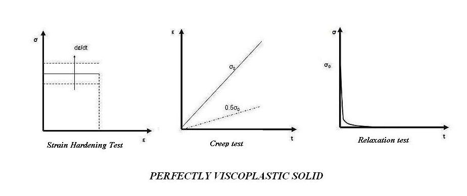
These models can be applied in metals and alloys at temperatures higher than one third of their absolute melting point (in kelvins) and polymers/asphalt at elevated temperature. The responses for strain hardening, creep, and relaxation tests of such material are shown in Figure 6.

Figure 6: The response of perfectly viscoplastic solid to hardening, creep and relaxation tests.

Elastic perfectly viscoplastic solid (Bingham-Norton model)

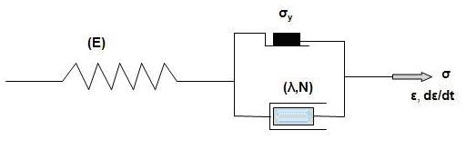
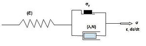Figure 7. The elastic perfectly viscoplastic material.

Two types of elementary approaches can be used to build up an elastic-perfectly viscoplastic mode. In the first situation, the sliding friction element and the dashpot are arranged in parallel and then connected in series to the elastic spring as shown in Figure 7. This model is called the Bingham-Maxwell model (by analogy with the Maxwell model and the Bingham model) or the Bingham-Norton model.^[22] In the second situation, all three elements are arranged in parallel. Such a model is called a Bingham-Kelvin model by analogy with the Kelvin model.

For elastic-perfectly viscoplastic materials, the elastic strain is no longer considered negligible but the rate of plastic strain is only a function of the initial yield stress and there is no influence of hardening. The sliding element represents a constant yielding stress when the elastic limit is exceeded irrespective of the strain. The model can be expressed as

$\begin{align} & \boldsymbol{\sigma} = \mathsf{E}~\boldsymbol{\varepsilon} & & \mathrm{for}~||\boldsymbol{\sigma}|| < \sigma_y \\ & \dot{\boldsymbol{\varepsilon}} = \dot{\boldsymbol{\varepsilon}}_{\mathrm{e}} + \dot{\boldsymbol{\varepsilon}}_{\mathrm{vp}} = \mathsf{E}^{-1}~\dot{\boldsymbol{\sigma}} + \cfrac{\boldsymbol{\sigma}}{\eta}\left[1 - \cfrac{\sigma_y}{||\boldsymbol{\sigma}||}\right] & & \mathrm{for}~||\boldsymbol{\sigma}|| \ge \sigma_y \end{align}$

where η is the viscosity of the dashpot element. If the dashpot element has a response that is of the Norton form

$\cfrac{\boldsymbol{\sigma}}{\eta} = \cfrac{\boldsymbol{\sigma}}{\lambda}\left[\cfrac{||\boldsymbol{\sigma}||}{\lambda}\right]^{N-1}$

we get the Bingham-Norton model

$\dot{\boldsymbol{\varepsilon}} = \mathsf{E}^{-1}~\dot{\boldsymbol{\sigma}} + \cfrac{\boldsymbol{\sigma}}{\lambda}\left[\cfrac{||\boldsymbol{\sigma}||}{\lambda}\right]^{N-1}\left[1 - \cfrac{\sigma_y}{||\boldsymbol{\sigma}||}\right] \quad \mathrm{for}~||\boldsymbol{\sigma}|| \ge \sigma_y$

Other expressions for the strain rate can also be observed in the literature^[22] with the general form

$\dot{\boldsymbol{\varepsilon}} = \mathsf{E}^{-1}~\dot{\boldsymbol{\sigma}} + f(\boldsymbol{\sigma}, \sigma_y)~\boldsymbol{\sigma} \quad \mathrm{for}~||\boldsymbol{\sigma}|| \ge \sigma_y$

The responses for strain hardening, creep, and relaxation tests of such material are shown in Figure 8.

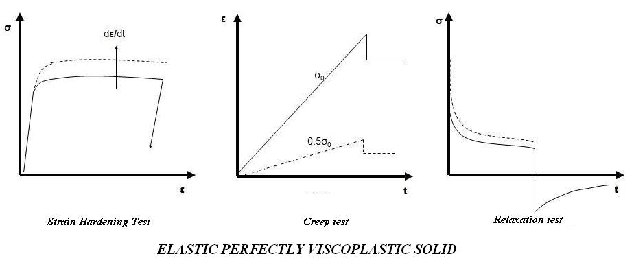
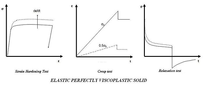Figure 8. The response of elastic perfectly viscoplastic solid to hardening, creep and relaxation tests.

Elastoviscoplastic hardening solid

An elastic-viscoplastic material with strain hardening is described by equations similar to those for a elastic-viscoplastic material with perfect plasticity. However, in this case the stress depends both on the plastic strain rate and on the plastic strain itself. For an elastoviscoplastic material the stress, after exceeding the yield stress, continues to increase beyond the initial yielding point. This implies that the yield stress in the sliding element increases with strain and the model may be expressed in generic terms as

$\begin{align} & \boldsymbol{\varepsilon} =\boldsymbol{\varepsilon}_{\mathrm{e}} = \mathsf{E}^{-1}~\boldsymbol{\sigma} = ~\boldsymbol{\varepsilon} & & \mathrm{for}~||\boldsymbol{\sigma}|| < \sigma_y \\ & \dot{\boldsymbol{\varepsilon}} = \dot{\boldsymbol{\varepsilon}}_{\mathrm{e}} + \dot{\boldsymbol{\varepsilon}}_{\mathrm{vp}} = \mathsf{E}^{-1}~\dot{\boldsymbol{\sigma}} + f(\boldsymbol{\sigma},\sigma_y,\boldsymbol{\varepsilon}_{\mathrm{vp}})~\boldsymbol{\sigma} & & \mathrm{for}~||\boldsymbol{\sigma}|| \ge \sigma_y \end{align}$.

This model is adopted when metals and alloys are at medium and higher temperatures and wood under high loads. The responses for strain hardening, creep, and relaxation tests of such a material are shown in Figure 9.

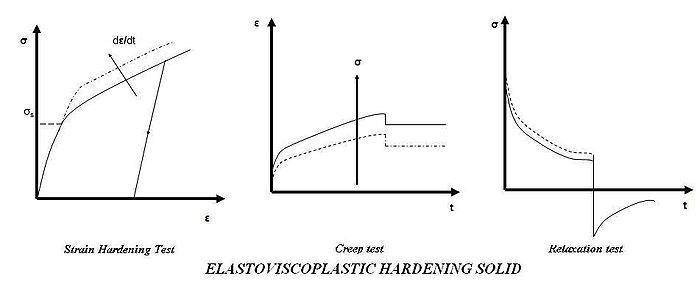Figure 9. The response of elastoviscoplastic hardening solid to hardening, creep and relaxation tests.

Strain-rate dependent plasticity models

Classical phenomenological viscoplasticity models for small strains are usually categorized into two types:^[3]

• the Perzyna formulation
• the Duvaut–Lions formulation

Perzyna formulation

In the Perzyna formulation the plastic strain rate is assumed to be given by a constitutive relation of the form

$\dot{\varepsilon}_{\mathrm{vp}} = \begin{cases} \cfrac{f(\boldsymbol{\sigma}, \boldsymbol{q})}{\tau} & \rm{if}~f(\boldsymbol{\sigma}, \boldsymbol{q}) > 0 \\ 0 & \rm{otherwise} \\ \end{cases}$

where f(.,.) is a yield function, $\boldsymbol{\sigma}$ is the Cauchy stress, $\boldsymbol{q}$ is a set of internal variables (such as the plastic strain $\boldsymbol{\varepsilon}_{\mathrm{vp}}$), τ is a relaxation time.

Duvaut–Lions formulation

The Duvaut–Lions formulation is equivalent to the Perzyna formulation and may be expressed as

$\dot{\varepsilon}_{\mathrm{vp}} = \begin{cases} \cfrac{\boldsymbol{\sigma} - \mathcal{P}\boldsymbol{\sigma}}{\tau} & \rm{if}~f(\boldsymbol{\sigma}, \boldsymbol{q}) > 0 \\ 0 & \rm{otherwise} \end{cases}$

where $\mathcal{P}\boldsymbol{\sigma}$ is the closest point projection of the stress state on to the boundary of the region that bounds all possible elastic stress states.

Flow stress models

The quantity $f(\boldsymbol{\sigma}, \boldsymbol{q})$ represents the evolution of the yield surface. The yield function f is often expressed as an equation consisting of some invariant of stress and a model for the yield stress (or plastic flow stress). An examaple is von Mises or J₂ plasticity. In those situations the plastic strain rate is calculated in the same manner as in rate-independent plasticity. In other situations, the yield stress model provides a direct means of computing the plastic strain rate.

Numerous empirical and semi-empirical flow stress models are used the computational plasticity. The following temperature and strain-rate dependent models provide a sampling of the models in current use:

1. the Johnson–Cook model
2. the Steinberg–Cochran–Guinan–Lund model.
3. the Zerilli–Armstrong model.
4. the Mechanical Threshold Stress model.
5. the Preston–Tonks–Wallace model.

The Johnson–Cook (JC) model ^[23] is purely empirical and is the most widely used of the five. However, this model exhibits an unrealistically small strain-rate dependence at high temperatures. The Steinberg–Cochran–Guinan–Lund (SCGL) model ^[24][25] is semi-empirical. The model is purely empirical and strain-rate independent at high strain-rates. A dislocation-based extension based on ^[26] is used at low strain-rates. The SCGL model is used extensively by the shock physics community. The Zerilli–Armstrong (ZA) model ^[27] is a simple physically based model that has been used extensively. A more complex model that is based on ideas from dislocation dynamics is the Mechanical Threshold Stress (MTS) model.^[28] This model has been used to model the plastic deformation of copper, tantalum,^[29] alloys of steel,^[30][31] and aluminum alloys.^[32] However, the MTS model is limited to strain-rates less than around 10⁷/s. The Preston–Tonks–Wallace (PTW) model ^[33] is also physically based and has a form similar to the MTS model. However, the PTW model has components that can model plastic deformation in the overdriven shock regime (strain-rates greater that 10⁷/s). Hence this model is valid for the largest range of strain-rates among the five flow stress models.

Johnson–Cook flow stress model

The Johnson–Cook (JC) model ^[23] is purely empirical and gives the following relation for the flow stress (σ_y)

$\text{(1)} \qquad \sigma_y(\varepsilon_{\rm{p}},\dot{\varepsilon_{\rm{p}}},T) = \left[A + B (\varepsilon_{\rm{p}})^n\right]\left[1 + C \ln(\dot{\varepsilon_{\rm{p}}}^{*})\right] \left[1 - (T^*)^m\right]$

where ε_p is the equivalent plastic strain, $\dot{\varepsilon_{\rm{p}}}$ is the plastic strain-rate, and A,B,C,n,m are material constants.

The normalized strain-rate and temperature in equation (1) are defined as

$\dot{\varepsilon_{\rm{p}}}^{*} := \cfrac{\dot{\varepsilon_{\rm{p}}}}{\dot{\varepsilon_{\rm{p0}}}} \qquad\text{and}\qquad T^* := \cfrac{(T-T_0)}{(T_m-T_0)}$

where $\dot{\varepsilon_{\rm{p0}}}$ is the effective plastic strain-rate of the quasi-static test used to determine the yield and hardening parameters A,B and n. This is not as it is often thought just a parameter to make $\dot{\varepsilon_{\rm{p}}}^{*}$ non-dimensional.^[34] T₀ is a reference temperature, and T_m is a reference melt temperature. For conditions where T ^* < 0, we assume that m = 1.

Steinberg–Cochran–Guinan–Lund flow stress model

The Steinberg–Cochran–Guinan–Lund (SCGL) model is a semi-empirical model that was developed by Steinberg et al.^[24] for high strain-rate situations and extended to low strain-rates and bcc materials by Steinberg and Lund.^[25] The flow stress in this model is given by

$\text{(2)} \qquad \sigma_y(\varepsilon_{\rm{p}},\dot{\varepsilon_{\rm{p}}},T) = \left[\sigma_a f(\varepsilon_{\rm{p}}) + \sigma_t (\dot{\varepsilon_{\rm{p}}}, T)\right] \frac{\mu(p,T)}{\mu_0}; \quad \sigma_a f \le \sigma_{\text{max}} ~~\text{and}~~ \sigma_t \le \sigma_p$

where σ_a is the athermal component of the flow stress, f(ε_p) is a function that represents strain hardening, σ_t is the thermally activated component of the flow stress, μ(p,T) is the pressure- and temperature-dependent shear modulus, and μ₀ is the shear modulus at standard temperature and pressure. The saturation value of the athermal stress is σ_max. The saturation of the thermally activated stress is the Peierls stress (σ_p). The shear modulus for this model is usually computed with the Steinberg–Cochran–Guinan shear modulus model.

The strain hardening function (f) has the form

f(ε_p) = [1 + β(ε_p + ε_pi)]ⁿ

where β,n are work hardening parameters, and ε_pi is the initial equivalent plastic strain.

The thermal component (σ_t) is computed using a bisection algorithm from the following equation.^[25][26]

$\dot{\varepsilon_{\rm{p}}} = \left[\frac{1}{C_1}\exp\left[\frac{2U_k}{k_b~T} \left(1 - \frac{\sigma_t}{\sigma_p}\right)^2\right] + \frac{C_2}{\sigma_t}\right]^{-1}; \quad \sigma_t \le \sigma_p$

where 2U_k is the energy to form a kink-pair in a dislocation segment of length L_d, k_b is the Boltzmann constant, σ_p is the Peierls stress. The constants C₁,C₂ are given by the relations

$C_1 := \frac{\rho_d L_d a b^2 \nu}{2 w^2}; \quad C_2 := \frac{D}{\rho_d b^2}$

where ρ_d is the dislocation density, L_d is the length of a dislocation segment, a is the distance between Peierls valleys, b is the magnitude of the Burgers vector, ν is the Debye frequency, w is the width of a kink loop, and D is the drag coefficient.

Zerilli–Armstrong flow stress model

The Zerilli–Armstrong (ZA) model ^[27][35][36] is based on simplified dislocation mechanics. The general form of the equation for the flow stress is

$\text{(3)} \qquad \sigma_y(\varepsilon_{\rm{p}},\dot{\varepsilon_{\rm{p}}},T) = \sigma_a + B\exp(-\beta(\dot{\varepsilon_{\rm{p}}}) T) + B_0\sqrt{\varepsilon_{\rm{p}}}\exp(-\alpha(\dot{\varepsilon_{\rm{p}}}) T) ~.$

In this model, σ_a is the athermal component of the flow stress given by

$\sigma_a := \sigma_g + \frac{k_h}{\sqrt{l}} + K\varepsilon_{\rm{p}}^n,$

where σ_g is the contribution due to solutes and initial dislocation density, k_h is the microstructural stress intensity, l is the average grain diameter, K is zero for fcc materials, B,B₀ are material constants.

In the thermally activated terms, the functional forms of the exponents α and β are

$\alpha = \alpha_0 - \alpha_1 \ln(\dot{\varepsilon_{\rm{p}}}); \quad \beta = \beta_0 - \beta_1 \ln(\dot{\varepsilon_{\rm{p}}});$

where α₀,α₁,β₀,β₁ are material parameters that depend on the type of material (fcc, bcc, hcp, alloys). The Zerilli–Armstrong model has been modified by ^[37] for better performance at high temperatures.

Mechanical threshold stress flow stress model

The Mechanical Threshold Stress (MTS) model ^[28][38][39]) has the form

$\text{(4)} \qquad \sigma_y(\varepsilon_{\rm{p}},\dot{\varepsilon_{\rm{p}}},T) = \sigma_a + (S_i \sigma_i + S_e \sigma_e)\frac{\mu(p,T)}{\mu_0}$

where σ_a is the athermal component of mechanical threshold stress, σ_i is the component of the flow stress due to intrinsic barriers to thermally activated dislocation motion and dislocation-dislocation interactions, σ_e is the component of the flow stress due to microstructural evolution with increasing deformation (strain hardening), (S_i,S_e) are temperature and strain-rate dependent scaling factors, and μ₀ is the shear modulus at 0 K and ambient pressure.

The scaling factors take the Arrhenius form

$\begin{align} S_i & = \left[1 - \left(\frac{k_b~T}{g_{0i}b^3\mu(p,T)} \ln\frac{\dot{\varepsilon_{\rm{p}}}}{\dot{\varepsilon_{\rm{p}}}}\right)^{1/q_i} \right]^{1/p_i} \\ S_e & = \left[1 - \left(\frac{k_b~T}{g_{0e}b^3\mu(p,T)} \ln\frac{\dot{\varepsilon_{\rm{p}}}}{\dot{\varepsilon_{\rm{p}}}}\right)^{1/q_e} \right]^{1/p_e} \end{align}$

where k_b is the Boltzmann constant, b is the magnitude of the Burgers' vector, (g_0i,g_0e) are normalized activation energies, ($\dot{\varepsilon_{\rm{p}}}, \dot{\varepsilon_{\rm{p}}}$) are constant reference strain-rates, and (q_i,p_i,q_e,p_e) are constants.

The strain hardening component of the mechanical threshold stress (σ_e) is given by an empirical modified Voce law

$\text{(5)} \qquad \frac{d\sigma_e}{d\varepsilon_{\rm{p}}} = \theta(\sigma_e)$

where

$\begin{align} \theta(\sigma_e) & = \theta_0 [ 1 - F(\sigma_e)] + \theta_{IV} F(\sigma_e) \\ \theta_0 & = a_0 + a_1 \ln \dot{\varepsilon_{\rm{p}}} + a_2 \sqrt{\dot{\varepsilon_{\rm{p}}}} - a_3 T \\ F(\sigma_e) & = \cfrac{\tanh\left(\alpha \cfrac{\sigma_e}{\sigma_{es}}\right)} {\tanh(\alpha)}\\ \ln(\cfrac{\sigma_{es}}{\sigma_{0es}}) & = \left(\frac{kT}{g_{0es} b^3 \mu(p,T)}\right) \ln\left(\cfrac{\dot{\varepsilon_{\rm{p}}}}{\dot{\varepsilon_{\rm{p}}}}\right) \end{align}$

and θ₀ is the hardening due to dislocation accumulation, θ_IV is the contribution due to stage-IV hardening, (a₀,a₁,a₂,a₃,α) are constants, σ_es is the stress at zero strain hardening rate, σ_0es is the saturation threshold stress for deformation at 0 K, g_0es is a constant, and $\dot{\varepsilon_{\rm{p}}}$ is the maximum strain-rate. Note that the maximum strain-rate is usually limited to about 10⁷/s.

Preston–Tonks–Wallace flow stress model

The Preston–Tonks–Wallace (PTW) model ^[33] attempts to provide a model for the flow stress for extreme strain-rates (up to 10¹¹/s) and temperatures up to melt. A linear Voce hardening law is used in the model. The PTW flow stress is given by

$\text{(6)} \qquad \sigma_y(\varepsilon_{\rm{p}},\dot{\varepsilon_{\rm{p}}},T) = \begin{cases} 2\left[\tau_s + \alpha\ln\left[1 - \varphi \exp\left(-\beta-\cfrac{\theta\varepsilon_{\rm{p}}}{\alpha\varphi}\right)\right]\right] \mu(p,T) & \text{thermal regime} \\ 2\tau_s\mu(p,T) & \text{shock regime} \end{cases}$

with

$\alpha := \frac{s_0 - \tau_y}{d}; \quad \beta := \frac{\tau_s - \tau_y}{\alpha}; \quad \varphi := \exp(\beta) - 1$

where τ_s is a normalized work-hardening saturation stress, s₀ is the value of τ_s at 0K, τ_y is a normalized yield stress, θ is the hardening constant in the Voce hardening law, and d is a dimensionless material parameter that modifies the Voce hardening law.

The saturation stress and the yield stress are given by

$\begin{align} \tau_s & = \max\left\{s_0 - (s_0 - s_{\infty}) \rm{erf}\left[\kappa \hat{T}\ln\left(\cfrac{\gamma\dot{\xi}}{\dot{\varepsilon_{\rm{p}}}}\right)\right], s_0\left(\cfrac{\dot{\varepsilon_{\rm{p}}}}{\gamma\dot{\xi}}\right)^{s_1}\right\} \\ \tau_y & = \max\left\{y_0 - (y_0 - y_{\infty}) \rm{erf}\left[\kappa \hat{T}\ln\left(\cfrac{\gamma\dot{\xi}}{\dot{\varepsilon_{\rm{p}}}}\right)\right], \min\left\{ y_1\left(\cfrac{\dot{\varepsilon_{\rm{p}}}}{\gamma\dot{\xi}}\right)^{y_2}, s_0\left(\cfrac{\dot{\varepsilon_{\rm{p}}}}{\gamma\dot{\xi}}\right)^{s_1}\right\}\right\} \end{align}$

where $s_{\infty}$ is the value of τ_s close to the melt temperature, ($y_0, y_{\infty}$) are the values of τ_y at 0 K and close to melt, respectively, (κ,γ) are material constants, $\hat{T} = T/T_m$, (s₁,y₁,y₂) are material parameters for the high strain-rate regime, and

$\dot{\xi} = \frac{1}{2}\left(\cfrac{4\pi\rho}{3M}\right)^{1/3} \left(\cfrac{\mu(p,T)}{\rho}\right)^{1/2}$

where ρ is the density, and M is the atomic mass.

See also

• Viscoelasticity
• Bingham plastic
• Dashpot
• Creep (deformation)
• Plasticity (physics)
• Continuum mechanics

References

1. ^ Perzyna, P. (1966). "Fundamental problems in viscoplasticity". Advances in applied mechanics 9 (2): 244–368. 
2. ^ J. Lemaitre and J. L. Chaboche (2002) "Mechanics of solid materials" Cambridge University Press.
3. ^ ^{a b c d} Simo, J.C.; Hughes, T.J.R. (1998), Computational inelasticity 
4. ^ Batra, R. C.; Kim, C. H. (1990). "Effect of viscoplastic flow rules on the initiation and growth of shear bands at high strain rates". Journal of the Mechanics and Physics of Solids 38 (6): 859–874. 
5. ^ Tresca, H. (1864). "Sur l'écoulement des Corps solides soumis à des fortes pressions". Comptes Rendus de l'Académie Sciences de Paris 59: 754–756. 
6. ^ Levy, M. (1871). "Extrait du mémoire sur les equations générales des mouvements intérieures des corps solides ductiles au dela des limites ou l'élasticité pourrait les ramener à leur premier état". J Math Pures Appl 16: 369–372. 
7. ^ Kojic, M. and Bathe, K-J., (2006), Inelastic Analysis of Solids and Structures, Elsevier.
8. ^ von Mises, R. (1913) "Mechanik der festen Korper im plastisch deformablen Zustand." Gottinger Nachr, math-phys Kl 1913:582–592.
9. ^ ^{a b c} Betten, J., 2005, Creep Mechanics: 2nd Ed., Springer.
10. ^ Norton, F. H. (1929). Creep of steel at high temperatures. McGraw-Hill Book Co., New York.
11. ^ Odqvist, F. K. G. (1934) "Creep stresses in a rotating disc." Proc. IV Int. Congress for Applied. Mechanics, Cambridge, p. 228.
12. ^ Prandtl, L. (1924) Proceedings of the 1st International Congress on Applied Mechanics, Delft.
13. ^ Reuss, A. (1930). "Berucksichtigung der elastichen, Formanderung in der Plastizitatstheorie". ZaMM 10: 266. 
14. ^ Hohenemser, K. and Prager, W., (1932), "Fundamental equations and definitions concerning the mechanics of isotropic continua,", J. Rheology, vol. 3.
15. ^ Bingham, E. C. (1922) Fluidity and plasticity. McGraw-Hill, New York.
16. ^ Hoff, ed., 1962, IUTAM Colloquium Creep in Structures; 1st, Stanford, Springer.
17. ^ Lubliner, J. (1990) Plasticity Theory, Macmillan Publishing Company, NY.
18. ^ Young, Mindness, Gray, ad Bentur (1998): "The Science and Technology of Civil Engineering Materials," Prentice Hall, NJ.
19. ^ François, D., Pineau, A., Zaoui, A., (1993), Mechanical Behaviour of Materials Volume II: Viscoplasticity, Damage, Fracture and Contact Mechanics, Kluwer Academic Publishers.
20. ^ Cristescu, N. and Gioda, G., (1994), Viscoplastic Behaviour of Geomaterials, International Centre for Mechanical Sciences.
21. ^ Rappaz, M., Bellet, M. and Deville, M., (1998), Numerical Modeling in Materials Science and Engineering, Springer.
22. ^ ^{a b} Irgens, F., (2008), Continuum Mechanics, Springer.
23. ^ ^{a b} Johnson, G.R.; Cook, W.H. (1983), "A constitutive model and data for metals subjected to large strains, high strain rates and high", Proceedings of the 7th International Symposium on Ballistics: 541–547, http://www.lajss.org/HistoricalArticles/A%20constitutive%20model%20and%20data%20for%20metals.pdf, retrieved 2009-05-13 
24. ^ ^{a b} Steinberg, D.J.; Cochran, S.G.; Guinan, M.W. (1980), "A constitutive model for metals applicable at high-strain rate", Journal of Applied Physics 51: 1498, doi:10.1063/1.327799 
25. ^ ^{a b c} Steinberg, D.J.; Lund, C.M. (1988), "A constitutive model for strain rates from 10⁻⁴ to 10⁶ s⁻¹", Journal de Physique. Colloques 49 (3): 3–3, http://cat.inist.fr/?aModele=afficheN, retrieved 2009-05-13 
26. ^ ^{a b} Hoge, K.G.; Mukherjee, A.K. (1977), "The temperature and strain rate dependence of the flow stress of tantalum", Journal of Materials Science 12 (8): 1666–1672, Bibcode 1977JMatS..12.1666H, doi:10.1007/BF00542818, http://www.springerlink.com/index/Q406613278W585P7.pdf, retrieved 2009-05-13 
27. ^ ^{a b} Zerilli, F.J.; Armstrong, R.W. (1987), "Dislocation-mechanics-based constitutive relations for material dynamics calculations", Journal of Applied Physics 61: 1816, doi:10.1063/1.338024 
28. ^ ^{a b} Follansbee, P.S.; Kocks, U.F. (1988), "A constitutive description of the deformation of copper based on the use of the mechanical threshold", Acta Metallurgica 36 (1): 81–93, doi:10.1016/0001-6160(88)90030-2 
29. ^ Chen, S.R.; Gray, G.T. (1996), "Constitutive behavior of tantalum and tantalum-tungsten alloys", Metallurgical and Materials Transactions A 27 (10): 2994–3006, Bibcode 1996MMTA...27.2994C, doi:10.1007/BF02663849, http://www.springerlink.com/index/D65G5112T720L7N5.pdf, retrieved 2009-05-13 
30. ^ Goto, D.M.; Garrett, R.K.; Bingert, J.F.; Chen, S.R.; Gray, G.T. (2000), "The mechanical threshold stress constitutive-strength model description of HY-100 steel", Metallurgical and Materials Transactions A 31 (8): 1985–1996, doi:10.1007/s11661-000-0226-8, http://www.springerlink.com/index/N4820676MU264G8H.pdf, retrieved 2009-05-13 
31. ^ Banerjee, B. (2007), "The Mechanical Threshold Stress model for various tempers of AISI 4340 steel", International Journal of Solids and Structures 44 (3–4): 834–859, arXiv:cond-mat/0510330, doi:10.1016/j.ijsolstr.2006.05.022 
32. ^ Puchi-cabrera, E.S.; Villalobos-gutierrez, C.; Castro-farinas, G. (2001), "On the mechanical threshold stress of aluminum: Effect of the alloying content", Journal of Engineering Materials and Technology 123: 155, doi:10.1115/1.1354990 
33. ^ ^{a b} Preston, D.L.; Tonks, D.L.; Wallace, D.C. (2003), "Model of plastic deformation for extreme loading conditions", Journal of Applied Physics 93: 211, doi:10.1063/1.1524706 
34. ^ Schwer http://www.dynalook.com/european-conf-2007/optional-strain-rate-forms-for-the-johnson-cook.pdf
35. ^ Zerilli, F.J.; Armstrong, R.W. (1994), "Constitutive relations for the plastic deformation of metals", AIP Conference Proceedings 309: 989, doi:10.1063/1.46201 
36. ^ Zerilli, F.J. (2004), "Dislocation mechanics-based constitutive equations", Metallurgical and Materials Transactions A 35 (9): 2547–2555, doi:10.1007/s11661-004-0201-x, http://www.springerlink.com/index/0406259680452456.pdf, retrieved 2009-05-13 
37. ^ Abed, F.H.; Voyiadjis, G.Z. (2005), "A consistent modified Zerilli–Armstrong flow stress model for BCC and FCC metals for elevated", Acta Mechanica 175 (1): 1–18, doi:10.1007/s00707-004-0203-1, http://www.springerlink.com/index/X7WFH0P2PJXK17FH.pdf, retrieved 2009-05-13 
38. ^ Goto, D.M.; Bingert, J.F.; Reed, W.R.; Garrett Jr, R.K. (2000), "Anisotropy-corrected MTS constitutive strength modeling in HY-100 steel", Scripta Materialia 42 (12): 1125–1131, doi:10.1016/S1359-6462(00)00347-X 
39. ^ Kocks, U.F. (2001), "Realistic constitutive relations for metal plasticity", Materials Science & Engineering A 317 (1–2): 181–187, doi:10.1016/S0921-5093(01)01174-1