- Nominal impedance
-
Nominal impedance in electrical engineering and audio engineering refers to the approximate designed impedance of an electrical circuit or device. The term is applied in a number of different fields, most often being encountered in respect of:
- The nominal value of the characteristic impedance of a cable of other form of transmission line.
- The nominal value of the input, output or image impedance of a port of a network, especially a network intended for use with a transmission line, such as filters, equalisers and amplifiers.
- The nominal value of the input impedance of a radio frequency antenna
The actual impedance may vary quite considerably from the nominal figure with changes in frequency. In the case of cables, there is also variation along the length of the cable. It is usual practice to speak of nominal impedance as if it were a constant resistance,[1] that is, it is invariant with frequency and has a zero reactive component, despite this often being far from the case. Depending on the field of application, nominal impedance is implicitly referring to a specific point on the frequency response of the circuit under consideration. This may be at low-frequency, mid-band or some other point and specific applications are discussed in the sections below.[2]
In most applications, there are a number of values of nominal impedance that are recognised as being standard. The nominal impedance of components and circuits are often assigned one of these standard values, regardless of whether the measured impedance exactly corresponds to it. The item is assigned the nearest standard value.
Contents
600 Ω
Nominal impedance first started to be specified in the early days of telecommunications. At first amplifiers were not available and when they did become available they were expensive. It was consequently necessary to squeeze every last drop of transmitted power from the cable at the receiving end in order to maximise the lengths of cables that could be installed. It also became apparent that reflections on the transmission line would severely limit the bandwidth that could be used or the distance that it was practicable to transmit. Matching equipment impedance to the characteristic impedance of the cable reduces reflections (and they are eliminated altogether if the match is perfect) and power transfer is maximised. To this end, all cables and equipment started to be specified to a standard nominal impedance. The earliest, and still the most widespread, standard is 600 Ω, originally used for telephony. It has to be said that the choice of this figure had more to do with the way telephones were interfaced into the local exchange than any characteristic of the local telephone cable. Telephones (old style analogue telephones) connect to the exchange through twisted pair cabling. Each leg of the pair is connected to a relay coil which detect the signalling on the line (dialling, handset off-hook etc). The other end of one coil is connected to volts and the second coil is connected to ground. A telephone exchange relay coil is around 300 Ω so the two of them together are terminating the line in 600 Ω.[3]
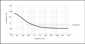 Variation of characteristic impedance with frequency. At audio frequencies the impedance is far from constant and the nominal value is only correct at one frequency.
The wiring to the subscriber in telephone networks is generally done in twisted pair cable. This format at audio frequencies, and especially at the more restricted telephone band frequencies, is far from constant. It is possible to manufacture this kind of cable to have a 600 Ω characteristic impedance but it will only be this value at one specific frequency. This might be quoted as a nominal 600 Ω impedance at 800 Hz or 1 kHz. Below this frequency the characteristic impedance rapidly rises and become more and more dominated by the ohmic resistance of the cable as the frequency falls. At the bottom of the audio band the impedance can be several tens of kilohms. On the other hand, at high frequency in the MHz region, the characteristic impedance flattens out to something almost constant. The reason for this response is explained at primary line constants.[4]
Local area networks (LANs) commonly use a similar kind of twisted pair cable, but screened and manufactured to tighter tolerances than is necessary for telephony. Even though it has a very similar impedance to telephone cable, the nominal impedance is rated at 100 Ω. This is because the LAN data is in a higher frequency band where the characteristic impedance is substantially flat and mostly resistive.[4]
Standardisation of line nominal impedance led to two-port networks such as filters being designed to a matching nominal impedance. The nominal impedance of low-pass symmetrical T- or Pi-filter sections (or more generally, image filter sections) is defined as the limit of the filter image impedance as the frequency approaches zero and is given by,
where L and C are as defined in constant k filter. As can be seen from the expression, this impedance is purley resistive. This filter transformed to a band-pass filter will have an impedance equal to the nominal impedance at resonance rather than low frequency. This nominal impedance of filters will generally be the same as the nominal impedance of the circuit or cable that the filter is working into.[5]
While 600 Ω is an almost universal standard in telephony for local presentation at customer's premises from the exchange, for long distance transmission on trunk lines between exchanges other standard nominal impedances are used and are usually lower, such as 150 Ω.[6]
50 Ω and 75 Ω
In the field of radio frequency (RF) and microwave engineering, by far and away the most common transmission line standard is 50 Ω coaxial cable (coax), which is an unbalanced line. 50 Ω first arose as a nominal impedance during world war two work on radar and is a compromise between two requirements. This standard was the work of the wartime US joint Army-Navy RF Cable Coordinating Committee. The first requirement is for minimum loss. The loss of coaxial cable is given by,
 nepers/metre
where R is the loop resistance per metre and Z0 is the characteristic impedance. Making the diameter of the inner conductor larger will decrease R and decreasing R decreases the loss. On the other hand, Z0 depends on the ratio of the diameters of outer and inner conductors (Dr) and will decrease with increasing inner conductor diameter thus increasing the loss. There is a specific value of Dr for which the loss is a minimum and this turns out to be 3.6. For an air dielectric coax (wartime coax was rigid air insulated pipe and this remained the case for some time afterwards) this corresponds to a characteristic impedance of 77 Ω. The second requirement is for maximum power handling and was an important requirement for radar. This is not the same condition as minimum loss because power handling is usually limited by the breakdown voltage of the dielectric. However, there is a similar compromise in terms of the ratio of conductor diameters. Making the inner conductor too large results in a thin insulator which breaks down at a lower voltage. On the other hand, making the inner conductor too small results in higher electric field strength near the inner conductor (because the field lines are closer together on the smaller circumference) and again reduces the breakdown voltage. The ideal ratio, Dr, for maximum power handling turns out to be 1.65 and corresponds to a characteristic impedance of 30 Ω in air. 50 Ω was arrived at by taking the geometric mean of these two figures;
and then rounding to a convenient whole number.[7][8]
Wartime production of coax, and for a period afterwards, tended to use standard plumbing pipe sizes for the outer conductor and standard AWG sizes for the inner conductor. This resulted in coax that was nearly, but not quite, 50 Ω. Matching is a much more critical requirement at RF than it is at voice frequencies, so when cable started to become available that was truly 50 Ω a need arose for matching circuits to interface between the new cables and legacy equipment, such as the rather strange 51.5 Ω to 50 Ω matching network.[8][9]
While 30 Ω cable is highly desirable for its power handling capabilities, it has never been in commercial production because the large size of inner conductor makes it difficult to manufacture. This is not the case with 77 Ω cable. 75 Ω nominal impedance cable has been in use from an early period in telecommunications for its low loss characteristic. According to Stephen Lampen of Belden Wire & Cable 75 Ω was chosen as the nominal impedance rather than 77 Ω because it corresponded to a standard AWG wire size for the inner conductor. 75 Ω is now the near universal standard nominal impedance for coaxial video interfaces and transmission lines.[8][10]
Radio antennae
The widespread idea that 50 Ω and 75 Ω nominal impedances are connected with the input impedance of various antennae is, in fact, a myth. It is true, however, that several common antennae are easily matched to these cables.[7] A quarter wavelength monopole has an impedance of 36.5 Ω,[11] and a half wavelength dipole has an impedance of 72 Ω.[12] A half-wavelength folded dipole, commonly seen on television antennae, on the other hand, has an impedance four times that of a dipole, that is 288 Ω. The 0.5λ dipole and the 0.5λ folded dipole are commonly taken as having nominal impedances of 75 Ω and 300 Ω respectively.[13]
Cable quality
One measure of cable manufacturing and installation quality is how closely the characteristic impedance adheres to the nominal impedance along its length. Impedance changes can be caused by variations in geometry along the cable length. In turn, these can be caused by a faulty manufacturing process or by faulty installation (such as not observing limits on bend radii). Unfortunately, there is no easy, non-destructive method of directly measuring impedance along a cables' length. It can, however, be indicated indirectly by measuring reflections, that is, return loss. Return loss by itself does not reveal much, since the cable design will have some intrinsic return loss anyway due to not having a purely resistive characteristic impedance. The technique used is to carefully adjust the cable termination to obtain as close a match as possible and then to measure the variation of return loss with frequency. The minimum return loss so measured is called the structural return loss (SRL). SRL is a measure of a cables' adherence to its nominal impedance but it is not a direct correspondence, errors further from the generator have less effect on SRL than those close to it. The measurement must also be carried out at all in-band frequencies to be significant. The reason for this is that equally spaced errors introduced by the manufacturing process will cancel and be invisible, or at least much reduced, at certain frequencies due to quarter wave impedance transformer action.[14][15]
Audio systems
For the most part, audio systems both professional and domestic, have their components interconnected with low impedance outputs connected to high impedance inputs. These impedances are poorly defined and nominal impedances are not usually assigned for this kind of connection. The exact impedances make little difference to performance as long as the latter is many times larger than the former.[16] This is a common interconnection scheme, not just for audio, but for electronic units in general which form part of a larger equipment or are only connected over a short distance. Where audio needs to be transmitted over large distances, which is often the case in broadcast engineering, considerations of matching and reflections dictate that a telecommunications standard is used, which would normally mean using 600 Ω nominal impedance (although other standards are sometimes encountered, such as sending at 75 Ω and receiving at 600 Ω which has bandwidth advantages). The nominal impedance of the transmission line and of the amplifiers and equalisers in the transmission chain will all be the same value.[6]
Nominal impedance is used, however, to characterise the transducers of an audio system, such as its microphones and loudspeakers. It is important that these are connected to a circuit capable of dealing with impedances in the appropriate range and assigning a nominal impedance is a convenient way of quickly determining likely incompatibilities. Loudspeakers and microphones are dealt with in separate sections below.
Loudspeakers
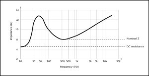 Diagram showing the variation in impedance of a typical mid-range loudspeaker. Nominal impedance is usually determined at the lowest point after resonance. However, it is possible for the low-frequency impedance to be still lower than this.[17]
Loudspeaker impedances are kept relatively low compared with other audio components so that the required audio power can be transmitted without using inconveniently (and dangerously) high voltages. The most common nominal impedance for loudspeakers is 8 Ω. Also used are 4 Ω and 16 Ω.[18] The once common 16 Ω is now mostly reserved for high frequency compression drivers since the high frequency end of the audio spectrum does not usually require so much power to reproduce.[19]
The impedance of a loudspeaker is not constant across all frequencies. In a typical loudspeaker the impedance will rise with increasing frequency from its dc value (see diagram) until it reaches a point of mechanical resonance. Following resonance, the impedance falls to a minimum and then begins to rise again.[20] Speakers are usually designed to operate at frequencies above their resonance, and for this reason it is the usual practice to define nominal impedance at this minimum and then round to the nearest standard value.[21][22] The ratio of the peak resonant frequency to the nominal impedance can be as much as 4:1.[23] It is, however, still perfectly possible for the low frequency impedance to actually be lower than the nominal impedance.[17] A given audio amplifier may not be capable of driving this low frequency impedance even though it is capable of driving the nominal impedance, a problem that can be solved either with the use of crossover filters or underrating the amplifier supplied.[24]
In the days of valves or vacuum tubes, most loudspeakers had a nominal impedance of 16 Ω. Valve outputs require an output transformer to match the very high output impedance and voltage of the output valves to this lower impedance. These transformers were commonly tapped to allow matching of the output to a multiple loudspeaker setup. For example, two 16 Ω loudspeakers in parallel will give an impedance of 8 Ω. Since the advent of solid-state transformerless outputs, these multiple-impedance outputs have become rare, and lower impedance loudspeakers more common. The most common nominal impedance for a single loudspeaker is now 8 Ω. Most solid-state amplifiers are designed to work with loudspeaker combinations of anything from 4 Ω to 8 Ω.[25]
Microphones
There are a large number of different types of microphone and there are correspondingly large differences in impedance between them. They range from the very low impedance of ribbon microphones (can be less than one ohm) to the very large impedance of piezoelectric microphones which are measured in megohms. The Electronic Industries Alliance (EIA) has defined[26] a number of standard microphone nominal impedances to aid categorisation of microphones.[27]
Range (Ω) EIA nominal impedance (Ω) 20-80 38 80-300 150 300-1250 600 1250-4500 2400 4500-20,000 9600 20,000-70,000 40,000 The International Electrotechnical Commission defines a similar set of nominal impedances, but also has a coarser classification of low, medium and high impedance with medium being 600 Ω to 10 kΩ.[28]
Oscilloscopes
Oscilloscope inputs are usually high impedance so that they only minimally affect the circuit being measured when connected. However, the input impedance is made a specific nominal value, rather than arbitrarily high, because of the common use of X10 probes. A common value for oscilloscope nominal impedance is 1 MΩ resistance and 20 pF capacitance.[29] With a known input impedance to the oscilloscope, the probe designer can ensure that the probe input impedance is exactly ten times this figure (actually oscilloscope plus probe cable impedance). Since the impedance included the input capacitance and the probe is an impedance divider circuit, the result is that the waveform being measured is not distorted by the RC circuit formed by the probe resistance and the capacitance of the input (or the cable capacitance which is generally higher).[30][31]
References
- ^ Maslin, p.78
- ^ Graf, p.506.
- ^ Schmitt, pp.301-302.
- ^ a b Schmitt, p.301.
- ^ Bird, pp.564, 569.
- ^ a b Whitaker, p.115.
- ^ a b Golio, p.6-41.
- ^ a b c Breed, pp.6-7.
- ^ Harmon Banning (W. L. Gore & Associates, Inc.), "The History of 50 Ω", RF Cafe
- ^ Steve Lampen, "Coax History" (mailing list), Contesting.com. Lampen is Technology Development Manager at Belden Wire & Cable Co. and is the author of Wire, Cable and Fiber Optics.
- ^ Chen, pp.574-575.
- ^ Gulati, p.424.
- ^ Gulati, p.426.
- ^ Rymaszewski et al, p.407.
- ^ Ciciora, p.435.
- ^ Eargle & Foreman, p.83.
- ^ a b Davis&Jones, p.205.
- ^ Ballou, p.523.
- ^ Vasey, pp.34-35.
- ^ Davis&Jones, p.206.
- ^ Davis&Jones, p.233.
- ^ Stark, p.200.
- ^ Davis&Jones, p.91.
- ^ Ballou, pp.523, 1178.
- ^ van der Veen, p.27.
- ^ Electronic Industries Standard SE-105, August 1949.
- ^ Ballou, p.419.
- ^ International standard IEC 60268-4 Sound system equipment - Part 4: Microphones.
- ^ pp.97-98.
- ^ Hickman, pp.33-37.
- ^ O'Dell, pp.72-79.
Bibliography
- Glen Ballou, Handbook for sound engineers, Gulf Professional Publishing, 2005 ISBN 0240807588.
- John Bird, Electrical circuit theory and technology, Elsevier, 2007 ISBN 075068139X.
- Gary Breed, "There's nothing magic about 50 ohms", High Frequency Electronics, pp. 6-7, June 2007, Summit Technical Media LLC.
- Wai-Kai Chen, The electrical engineering handbook, Academic Press, 2005 ISBN 0121709604.
- Walter S. Ciciora, Modern cable television technology: video, voice, and data communications, Morgan Kaufmann, 2004 ISBN 1558608281.
- Gary Davis, Ralph Jones, The sound reinforcement handbook, Hal Leonard Corporation, 1989 ISBN 0881889008.
- John Eargle, Chris Foreman, Audio engineering for sound reinforcement, Hal Leonard Corporation, 2002, ISBN 0634043552.
- John Michael Golio, The RF and microwave handbook, CRC Press, 2001 ISBN 084938592X.
- Rudolf F. Graf, Modern dictionary of electronics, Newnes, 1999 ISBN 0750698667.
- R.R. Gulati, Modern Television Practice Principles,Technology and Servicing, New Age International, ISBN 8122413609.
- Ian Hickman, Oscilloscopes: how to use them, how they work, Newnes, 2001 ISBN 0750647574.
- Stephen Lampen, Wire, Cable and Fiber Optics for Video and Audio Engineers, McGraw-Hill 1997 ISBN 0070381348.
- A.K.Maini, Electronic Projects For Beginners, Pustak Mahal, 1997 ISBN 8122301525.
- Nicholas M. Maslin, HF communications: a systems approach, CRC Press, 1987 ISBN 0273026755.
- Thomas Henry O'Dell, Circuits for electronic instrumentation, Cambridge University Press, 1991 ISBN 0521404282.
- R. Tummala, E. J. Rymaszewski (ed), Alan G. Klopfenstein, Microelectronics packaging handbook, Volume 3, Springer, 1997 ISBN 0412084511.
- Ron Schmitt, Electromagnetics explained: a handbook for wireless/RF, EMC, and high-speed electronics, Newnes, 2002 ISBN 0750674032.
- Scott Hunter Stark, Live sound reinforcement: a comprehensive guide to P.A. and music reinforcement systems and technology, Hal Leonard Corporation, 1996 ISBN 0918371074.
- John Vasey, Concert sound and lighting systems, Focal Press, 1999 ISBN 0240803647.
- Menno van der Veen, Modern high-end valve amplifiers: based on toroidal output transformers, Elektor International Media, 1999 ISBN 0905705637.
- Jerry C. Whitaker, Television receivers, McGraw-Hill Professional, 2001 ISBN 0071380426.
Categories:- Electrical parameters


Wikimedia Foundation. 2010.