Distribution (mathematics)

This article is about generalized functions in mathematical analysis. For the probability meaning, see Probability distribution. For other uses, see Distribution (disambiguation).

In mathematical analysis, distributions (or generalized functions) are objects that generalize functions. Distributions make it possible to differentiate functions whose derivatives do not exist in the classical sense. In particular, any locally integrable function has a distributional derivative. Distributions are widely used to formulate generalized solutions of partial differential equations. Where a classical solution may not exist or be very difficult to establish, a distribution solution to a differential equation is often much easier. Distributions are also important in physics and engineering where many problems naturally lead to differential equations whose solutions or initial conditions are distributions, such as the Dirac delta distribution.

Generalized functions were introduced by Sergei Sobolev in 1935. They were re-introduced in the late 1940s by Laurent Schwartz, who developed a comprehensive theory of distributions.

Basic idea

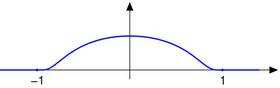A typical test function, the bump function Ψ(x). It is smooth (infinitely differentiable) and has compact support (is zero outside an interval, in this case the interval [-1, 1]).

Distributions are a class of linear functionals that map a set of test functions (conventional and well-behaved functions) onto the set of real numbers. In the simplest case, the set of test functions considered is D(R), which is the set of functions from R to R having two properties:

• The function is smooth (infinitely differentiable);
• The function has compact support (is identically zero outside some interval).

Then, a distribution d is a linear mapping from D(R) to R. Instead of writing d(φ), where φ is a test function in D(R), it is conventional to write $\langle d, \varphi\rangle$. A simple example of a distribution is the Dirac delta δ, defined by

$\delta(\varphi) = \left\langle \delta, \varphi \right\rangle = \varphi(0).$

There are straightforward mappings from both locally integrable functions and probability distributions to corresponding distributions, as discussed below. However, not all distributions can be formed in this manner.

Suppose that

$f: \mathbf{R} \rightarrow \mathbf{R}$

is a locally integrable function, and let

$\varphi: \mathbf{R} \rightarrow \mathbf{R}$

be a test function in D(R). We can then define a corresponding distribution T_f by:

$\left\langle T_f, \varphi \right\rangle = \int_\mathbf{R} f \varphi \,dx$.

This integral is a real number which linearly and continuously depends on φ. This suggests the requirement that a distribution should be linear and continuous over the space of test functions D(R), which completes the definition. In a conventional abuse of notation, f may be used to represent both the original function f and the distribution T_f derived from it.

Similarly, if P is a probability distribution on the reals and φ is a test function, then a corresponding distribution T_P may be defined by:

$\left\langle T_P, \varphi \right\rangle = \int_{\mathbf{R}} \varphi\, dP$

Again, this integral continuously and linearly depends on φ, so that T_P is in fact a distribution.

Such distributions may be multiplied with real numbers and can be added together, so they form a real vector space. In general it is not possible to define a multiplication for distributions, but distributions may be multiplied with infinitely differentiable functions.

It's desirable to choose a definition for the derivative of a distribution which, at least for distributions derived from locally integrable functions, has the property that (T_f)' = T_{f '}. If φ is a test function, we can show that

$\left\langle T_{f'}, \varphi\right\rangle = \int_{\mathbf{R}}{}{f'\varphi \,dx} = - \int_{\mathbf{R}}{}{f\varphi' \,dx} = -\left\langle T_f, \varphi' \right\rangle$

using integration by parts and noting that $\left[ f(x) \varphi(x) \right]_{-\infty}^\infty = 0$, since φ is zero outside of a bounded set. This suggests that if S is a distribution, we should define its derivative S' by

$\left\langle S', \varphi \right\rangle = - \left\langle S, \varphi' \right\rangle$.

It turns out that this is the proper definition; it extends the ordinary definition of derivative, every distribution becomes infinitely differentiable and the usual properties of derivatives hold.

Example: Recall that the Dirac delta (so-called Dirac delta function) is the distribution defined by

$\left\langle \delta, \varphi \right\rangle = \varphi(0)$

It is the derivative of the distribution corresponding to the Heaviside step function H: For any test function φ,

$\left\langle (T_H)', \varphi \right\rangle = - \left\langle T_H, \varphi' \right\rangle = - \int_{-\infty}^{\infty} H(x) \varphi'(x) dx =$

$= - \int_{0}^{\infty} \varphi'(x) dx = \varphi(0) - \varphi(\infty) = \varphi(0) = \left\langle \delta, \varphi \right\rangle,$

so (T_H)' = δ. Note, $\varphi(\infty)=0$ because of compact support. Similarly, the derivative of the Dirac delta is the distribution

$\langle\delta',\varphi\rangle= -\varphi'(0).$

This latter distribution is our first example of a distribution which is derived from neither a function nor a probability distribution.

Test functions and distributions

In the sequel, real-valued distributions on an open subset U of Rⁿ will be formally defined. With minor modifications, one can also define complex-valued distributions, and one can replace Rⁿ by any (paracompact) smooth manifold.

The first object to define is the space D(U) of test functions on U. Once this is defined, it is then necessary to equip it with a topology by defining the limit of a sequence of elements of D(U). The space of distributions will then be given as the space of continuous linear functionals on D(U).

Test function space

The space D(U) of test functions on U is defined as follows. A function φ : U → R is said to have compact support if there exists a compact subset K of U such that φ(x) = 0 for all x in U \ K. The elements of D(U) are the infinitely differentiable functions φ : U → R with compact support – also known as bump functions. This is a real vector space. It can be given a topology by defining the limit of a sequence of elements of D(U). A sequence (φ_k) in D(U) is said to converge to φ ∈ D(U) if the following two conditions hold (Gelfand & Shilov 1966–1968, v. 1, §1.2):

• There is a compact set K ⊂ U containing the supports of all φ_k:

$\bigcup_k \operatorname{supp}(\varphi_k)\subset K.$

• For each multiindex α, the sequence of partial derivatives D^αφ_k tends uniformly to D^αφ.

With this definition, D(U) becomes a complete locally convex topological vector space satisfying the Heine–Borel property (Rudin 1991, §6.4-5). If U_i is a countable nested family of open subsets of U with compact closures $\scriptstyle{K_i = \bar{U}_i}$, then

$\mathrm{D}(U) = \bigcup_i \mathrm{D}_{K_i}$

where D_Ki is the set of all smooth functions with support lying in K_i. The topology on D(U) is the final topology of the family of nested metric spaces D_Ki and so D(U) is an LF-space. The topology is not metrizable by the Baire category theorem, since D(U) is the union of subspaces of the first category in D(U) (Rudin 1991, §6.9).

Distributions

A distribution on U is a linear functional S : D(U) → R (or S : D(U) → C), such that

$\lim_{n\to\infty}S(\varphi_n)= S\left(\lim_{n\to\infty}\varphi_n\right)$

for any convergent sequence φ_n in D(U). The space of all distributions on U is denoted by D'(U). Equivalently, the vector space D'(U) is the continuous dual space of the topological vector space D(U).

The dual pairing between a distribution S in D′(U) and a test function 'φ' in D(U) is denoted using angle brackets thus:

$\mathrm{D}'(U) \times \mathrm{D}(U) \ni (S, \varphi) \mapsto \langle S, \varphi \rangle \in \mathbf{R}.$

Equipped with the weak-* topology, the space D'(U) is a locally convex topological vector space. In particular, a sequence (S_k) in D'(U) converges to a distribution S if and only if

$\langle S_k, \varphi\rangle \to \langle S, \varphi\rangle$

for all test functions φ. This is the case if and only if S_k converges uniformly to S on all bounded subsets of D(U). (A subset E of D(U) is bounded if there exists a compact subset K of U and numbers d_n such that every φ in E has its support in K and has its n-th derivatives bounded by d_n.)

Functions as distributions

The function ƒ : U → R is called locally integrable if it is Lebesgue integrable over every compact subset K of U. This is a large class of functions which includes all continuous functions and all L^p functions. The topology on D(U) is defined in such a fashion that any locally integrable function ƒ yields a continuous linear functional on D(U) – that is, an element of D′(U) – denoted here by T_ƒ, whose value on the test function φ is given by the Lebesgue integral:

$\langle T_f,\varphi \rangle = \int_U f\varphi\,dx.$

Conventionally, one abuses notation by identifying T_ƒ with ƒ, provided no confusion can arise, and thus the pairing between ƒ and φ is often written

$\langle f, \varphi\rangle = \langle T_f,\varphi\rangle.$

If ƒ and g are two locally integrable functions, then the associated distributions T_ƒ and T_g are equal to the same element of D'(U) if and only if ƒ and g are equal almost everywhere (see, for instance, Hörmander (1983, Theorem 1.2.5)). In a similar manner, every Radon measure μ on U defines an element of D'(U) whose value on the test function φ is ∫φ dμ. As above, it is conventional to abuse notation and write the pairing between a Radon measure μ and a test function φ as $\scriptstyle{\langle\mu,\varphi\rangle}$. Conversely, essentially by the Riesz representation theorem, every distribution which is non-negative on non-negative functions is of this form for some (positive) Radon measure.

The test functions are themselves locally integrable, and so define distributions. As such they are dense in D'(U) with respect to the topology on D'(U) in the sense that for any distribution S ∈ D'(U), there is a sequence φ_n ∈ D(U) such that

$\langle\varphi_n,\psi\rangle\to \langle S,\psi\rangle$

for all ψ ∈ D(U). This follows at once from the Hahn–Banach theorem, since by an elementary fact about weak topologies the dual of D'(U) with its weak-* topology is the space D(U) (Rudin 1991, Theorem 3.10). This can also be proven more constructively by a convolution argument.

Operations on distributions

Many operations which are defined on smooth functions with compact support can also be defined for distributions. In general, if

$T : \mathrm{D}(U) \to \mathrm{D}(U)$

is a linear mapping of vector spaces which is continuous with respect to the weak-* topology, then it is possible to extend T to a mapping

$T : \mathrm{D}'(U) \to \mathrm{D}'(U)$

by passing to the limit. (This approach works for more general non-linear mappings as well, provided they are assumed to be uniformly continuous.)

In practice, however, it is more convenient to define operations on distributions by means of the transpose (or adjoint transformation) (Strichartz 1994, §2.3; Trèves 1967). If T : D(U) → D(U) is a continuous linear operator, then the transpose is an operator T^* : D(U) → D(U) such that

$\langle T\varphi,\psi\rangle = \langle\varphi, T^*\psi\rangle$

for all φ, ψ ∈ D(U). If such an operator T^* exists, and is continuous, then the original operator T may be extended to distributions by defining

$Tf(\psi) = f(T^*\psi).\,$

Differentiation

If T : D(U) → D(U) is given by the partial derivative

$T\varphi = \frac{\partial\varphi}{\partial x_k}.$

By integration by parts, if φ and ψ are in D(U), then

$\langle T\varphi,\psi\rangle=\left\langle\frac{\partial\varphi}{\partial x_k},\psi\right\rangle = -\left\langle\varphi,\frac{\partial\psi}{\partial x_k}\right\rangle$

so that T^* = −T. This is a continuous linear transformation D(U) → D(U). So, if S ∈ D'(U) is a distribution, then the partial derivative of S with respect to the coordinate x_k is defined by the formula

$\left\langle \frac{\partial S}{\partial x_{k}}, \varphi \right\rangle = - \left\langle S, \frac{\partial \varphi}{\partial x_{k}} \right\rangle$

for all test functions 'φ'. In this way, every distribution is infinitely differentiable, and the derivative in the direction x_k is a linear operator on D′(U). In general, if α = (α₁, ..., α_n) is an arbitrary multi-index and ∂^α denotes the associated mixed partial derivative operator, the mixed partial derivative ∂^αS of the distribution S ∈ D′(U) is defined by

$\left\langle \partial^{\alpha} S, \varphi \right\rangle = (-1)^{| \alpha |} \left\langle S, \partial^{\alpha} \varphi \right\rangle \mbox{ for all } \varphi \in \mathrm{D}(U).$

Differentiation of distributions is a continuous operator on D'(U); this is an important and desirable property that is not shared by most other notions of differentiation.

Multiplication by a smooth function

If m : U → R is an infinitely differentiable function and S is a distribution on U, then the product mS is defined by (mS)(φ) = S(mφ) for all test functions φ. This definition coincides with the transpose transformation of

$T_m : \varphi\mapsto m\varphi$

for φ ∈ D(U). Then, for any test function ψ

$\langle T_m\varphi,\psi\rangle = \int_U m(x)\varphi(x)\psi(x)\,dx = \langle\varphi, T_m\psi\rangle$

so that T_m^* = T_m. Multiplication of a distribution S by the smooth function m is therefore defined by

$mS(\psi) = \langle mS, \psi\rangle = \langle S, m\psi\rangle = S(m\psi).$

Under multiplication by smooth functions, D'(U) is a module over the ring C^∞(U). With this definition of multiplication by a smooth function, the ordinary product rule of calculus remains valid. However, a number of unusual identities also arise. For example, the Dirac delta distribution δ is defined on R by 〈δ, φ〉 = φ(0), so that mδ = m(0)δ. Its derivative is given by〈δ', φ〉 = −〈δ, φ〉 = −φ(0). But the product mδ' of m and δ' is the distribution

$m\delta' = m(0)\delta' - m'\delta = m(0)\delta' - m'(0)\delta.\,$

This definition of multiplication also makes it possible to define the operation of a linear differential operator with smooth coefficients on a distribution. A linear differential operator takes a distribution S ∈ D'(U) to another distribution given by a sum of the form

$PS = \sum_{|\alpha|\le k} p_\alpha \partial^\alpha S$

where the coefficients p_α are smooth functions in U. If P is a given differential operator, then the minimum integer k for which such an expansion holds for every distribution S is called the order of P. The transpose of P is given by

$\left\langle \sum_\alpha p_\alpha \partial^\alpha S,\varphi\right\rangle = \left\langle S,\sum_\alpha (-1)^{|\alpha|} \partial^\alpha(p_\alpha\varphi)\right\rangle.$

The space D'(U) is a D-module with respect to the action of the ring of linear differential operators.

Composition with a smooth function

Let S be a distribution on an open set U ⊂ Rⁿ. Let V be an open set in Rⁿ, and F : V → U. Then provided F is a submersion, it is possible to define

$S\circ F \in \mathrm{D}'(V).$

This is the composition of the distribution S with F, and is also called the pullback of S along F, sometimes written

$F^\sharp : S\mapsto F^\sharp S = S\circ F.$

The pullback is often denoted F^*, but this notation risks confusion with the above use of '*' to denote the transpose of a linear mapping.

The condition that F be a submersion is equivalent to the requirement that the Jacobian derivative dF(x) of F is a surjective linear map for every x ∈ V. A necessary (but not sufficient) condition for extending F^# to distributions is that F be an open mapping (Hörmander 1983, Theorem 6.1.1). The inverse function theorem ensures that a submersion satisfies this condition.

If F is a submersion, then F^# is defined on distributions by finding the transpose map. Uniqueness of this extension is guaranteed since F^# is a continuous linear operator on D(U). Existence, however, requires using the change of variables formula, the inverse function theorem (locally) and a partition of unity argument; see Hörmander (1983, Theorem 6.1.2).

In the special case when F is a diffeomorphism from an open subset V of Rⁿ onto an open subset U of Rⁿ change of variables under the integral gives

$\int_V\varphi\circ F(x) \psi(x)\,dx = \int_U\varphi(x)\psi(F^{-1}(x))|\det dF^{-1}(x)|\,dx.$

In this particular case, then, F^# is defined by the transpose formula:

$\langle F^\sharp S,\varphi \rangle = \langle S,|\det d(F^{-1})| \varphi\circ F^{-1}\rangle.$

Localization of distributions

There is no way to define the value of a distribution in D'(U) at a particular point of U. However, as is the case with functions, distributions on U restrict to give distributions on open subsets of U. Furthermore, distributions are locally determined in the sense that a distribution on all of U can be assembled from a distribution on an open cover of U satisfying some compatibility conditions on the overlap. Such a structure is known as a sheaf.

Restriction

Let U and V be open subsets of Rⁿ with V ⊂ U. Let E_VU : D(V) → D(U) be the operator which extends by zero a given smooth function compactly supported in V to a smooth function compactly supported in the larger set U. Then the restriction mapping ρ _VU is defined to be the transpose of E_VU. Thus for any distribution S ∈ D'(U), the restriction ρ_VU S is a distribution in the dual space D'(V) defined by

$\langle \rho_{VU}S,\varphi\rangle = \langle S, E_{VU}\varphi\rangle$

for all test functions φ ∈ D(V).

Unless U = V, the restriction to V is neither injective nor surjective. Lack of surjectivity follows since distributions can blow up towards the boundary of V. For instance, if U = R and V = (0,2), then the distribution

$S(x) = \sum_{n=1}^\infty n\,\delta\left(x-\frac{1}{n}\right)$

is in D'(V) but admits no extension to D'(U).

Support of a distribution

Let S ∈ D′(U) be a distribution on an open set U. Then S is said to vanish on an open set V of U if S lies in the kernel of the restriction map ρ_VU. Explicitly S vanishes on V if

$\langle S,\varphi\rangle = 0$

for all test functions φ ∈ C^∞(U) with support in V. Let V be a maximal open set on which the distribution S vanishes; i.e., V is the union of every open set on which S vanishes. The support of S is the complement of V in U. Thus

$\operatorname{supp}\,S = U - \bigcup\left\{V \mid \rho_{VU}S = 0\right\}.$

The distribution S has compact support if its support is a compact set. Explicitly, S has compact support if there is a compact subset K of U such that for every test function φ whose support is completely outside of K, we have S(φ) = 0. Compactly supported distributions define continuous linear functions on the space C^∞(U); the topology on C^∞(U) is defined such that a sequence of test functions φ_k converges to 0 if and only if all derivatives of φ_k converge uniformly to 0 on every compact subset of U. Conversely, it can be shown that every continuous linear functional on this space defines a distribution of compact support.

Tempered distributions and Fourier transform

By using a larger space of test functions, one can define the tempered distributions, a subspace of D'(Rⁿ). These distributions are useful if one studies the Fourier transform in generality: all tempered distributions have a Fourier transform, but not all distributions have one.

The space of test functions employed here, the so-called Schwartz space S(Rⁿ), is the function space of all infinitely differentiable functions that are rapidly decreasing at infinity along with all partial derivatives. Thus φ : Rⁿ → R is in the Schwartz space provided that any derivative of φ, multiplied with any power of |x|, converges towards 0 for |x| → ∞. These functions form a complete topological vector space with a suitably defined family of seminorms. More precisely, let

$p_{\alpha , \beta} (\varphi) = \sup_{x \in \mathbf{R}^n} | x^\alpha D^\beta \varphi(x)|$

for α, β multi-indices of size n. Then φ is a Schwartz function if all the values

$p_{\alpha, \beta} (\varphi) < \infty.$

The family of seminorms p_{α, β} defines a locally convex topology on the Schwartz-space. The seminorms are, in fact, norms on the Schwartz space, since Schwartz functions are smooth. The Schwartz space is metrizable and complete. Because the Fourier transform changes differentiation by x^α into multiplication by x^α and vice-versa, this symmetry implies that the Fourier transformations of a Schwartz function is also a Schwartz function.

The space of tempered distributions is defined as the (continuous) dual of the Schwartz space. In other words, a distribution F is a tempered distribution if and only if

$\lim_{m\to\infty} F(\varphi_m)=0.$

is true whenever,

$\lim_{m\to\infty} p_{\alpha , \beta} (\varphi_m) = 0$

holds for all multi-indices α, β.

The derivative of a tempered distribution is again a tempered distribution. Tempered distributions generalize the bounded (or slow-growing) locally integrable functions; all distributions with compact support and all square-integrable functions are tempered distributions. All locally integrable functions ƒ with at most polynomial growth, i.e. such that ƒ(x) = O(|x|^r) for some r, are tempered distributions. This includes all functions in L^p(Rⁿ) for p ≥ 1.

The tempered distributions can also be characterized as slowly growing. This characterization is dual to the rapidly falling behaviour, e.g. $\propto |x|^n \cdot \exp (- x^2)$, of the test functions.

To study the Fourier transform, it is best to consider complex-valued test functions and complex-linear distributions. The ordinary continuous Fourier transform F yields then an automorphism of Schwartz function space, and we can define the Fourier transform of the tempered distribution S by (FS)(ψ) = S(Fψ) for every test function ψ.   FS is thus again a tempered distribution. The Fourier transform is a continuous, linear, bijective operator from the space of tempered distributions to itself. This operation is compatible with differentiation in the sense that

$F\dfrac{dS}{dx}=ixFS$

and also with convolution: if S is a tempered distribution and ψ is a slowly increasing infinitely differentiable function on Rⁿ (meaning that all derivatives of ψ grow at most as fast as polynomials), then Sψ is again a tempered distribution and

$F(S\psi)=FS*F\psi\,$

is the convolution of FS and Fψ. In particular, the Fourier transform of the unity function is the δ distribution.

Convolution

Under some circumstances, it is possible to define the convolution of a function with a distribution, or even the convolution of two distributions.

Convolution of a test function with a distribution

If ƒ ∈ D(Rⁿ) is a compactly supported smooth test function, then convolution with ƒ defines an operator

$C_f : D(\mathbf{R}^n)\to D(\mathbf{R}^n)$

defined by C_ƒg = ƒ∗g, which is linear (and continuous with respect to the LF space topology on D(Rⁿ).)

Convolution of ƒ with a distribution S ∈ D′(Rⁿ) can be defined by taking the transpose of C_ƒ relative to the duality pairing of D(Rⁿ) with the space D′(Rⁿ) of distributions (Trèves 1967, Chapter 27). If ƒ, g,  'φ' ∈ D(Rⁿ), then by Fubini's theorem

$\langle C_fg, \varphi\rangle = \int_{\mathbf{R}^n}\varphi(x)\int_{\mathbf{R}^n}f(x-y)g(y)\,dydx = \langle g, C_{\tilde{f}}\varphi\rangle$

where $\scriptstyle{\tilde{f}(x) = f(-x)}$. Extending by continuity, the convolution of ƒ with a distribution S is defined by

$\langle f*S, \varphi\rangle = \langle S, \tilde{f}*\varphi\rangle$

for all test functions 'φ' ∈ D(Rⁿ).

An alternative way to define the convolution of a function ƒ and a distribution S is to use the translation operator τ_x defined on test functions by

τ_xφ(y) = φ(y − x)

and extended by the transpose to distributions in the obvious way (Rudin 1991, §6.29). The convolution of the compactly supported function ƒ and the distribution S is then the function defined for each x ∈ Rⁿ by

$(f*S)(x) = \langle S, \tau_x\tilde{f}\rangle.$

It can be shown that the convolution of a compactly supported function and a distribution is a smooth function. If the distribution S has compact support as well, then ƒ∗S is a compactly supported function, and the Titchmarsh convolution theorem (Hörmander 1983, Theorem 4.3.3) implies that

$\operatorname{ch}(f*S) = \operatorname{ch}f + \operatorname{ch}S$

where ch denotes the convex hull.

Distribution of compact support

It is also possible to define the convolution of two distributions S and T on Rⁿ, provided one of them has compact support. Informally, in order to define S∗T where T has compact support, the idea is to extend the definition of the convolution ∗ to a linear operation on distributions so that the associativity formula

S * (T * φ) = (S * T) * φ

continues to hold for all test-functions 'φ'. Hörmander (1983, §IV.2) proves the uniqueness of such an extension.

It is also possible to provide a more explicit characterization of the convolution of distributions (Trèves 1967, Chapter 27). Suppose that it is T that has compact support. For any test function 'φ' in D(Rⁿ), consider the function

$\psi(x) = \langle T, \tau_{-x}\varphi\rangle.$

It can be readily shown that this defines a smooth function of x, which moreover has compact support. The convolution of S and T is defined by

$\langle S * T,\varphi\rangle = \langle S, \psi\rangle.$

This generalizes the classical notion of convolution of functions and is compatible with differentiation in the following sense:

$\partial^\alpha(S*T)=(\partial^\alpha S)*T=S*(\partial^\alpha T).$

This definition of convolution remains valid under less restrictive assumptions about S and T; see for instance Gel'fand & Shilov (1966–1968, v. 1, pp. 103–104) and Benedetto (1997, Definition 2.5.8).

Distributions as derivatives of continuous functions

The formal definition of distributions exhibits them as a subspace of a very large space, namely the topological dual of D(U) (or S(R^d) for tempered distributions). It is not immediately clear from the definition how exotic a distribution might be. To answer this question, it is instructive to see distributions built up from a smaller space, namely the space of continuous functions. Roughly, any distribution is locally a (multiple) derivative of a continuous function. A precise version of this result, given below, holds for distributions of compact support, tempered distributions, and general distributions. Generally speaking, no proper subset of the space of distributions contains all continuous functions and is closed under differentiation. This says that distributions are not particularly exotic objects; they are only as complicated as necessary.

Tempered distributions

If ƒ ∈ S′(Rⁿ) is a tempered distribution, then there exists a constant C > 0, and positive integers M and N such that for all Schwartz functions φ ∈S(Rⁿ)

$\langle f, \varphi\rangle \le C\sum_{|\alpha|\le N, |\beta|\le M}\sup_{x\in\mathbf{R}^n}|x^\alpha D^\beta \varphi(x)|=C\sum_{|\alpha|\le N, |\beta|\le M}p_{\alpha,\beta}(\varphi).$

This estimate along with some techniques from functional analysis can be used to show that there is a continuous slowly increasing function F and a multiindex α such that

$f=D^\alpha F.\,$

Compactly supported distributions

Let U be an open set, and K a compact subset of U. If ƒ is a distribution supported on K, then there is a continuous function F compactly supported in U (possibly on a larger set than K itself) such that

$f = D^\alpha F\,$

for some multi-index α. This follows from the previously quoted result on tempered distributions by means of a localization argument.

Distributions with point support

If ƒ has support at a single point {P}, then ƒ is in fact a finite linear combination of distributional derivatives of the δ function at P. That is, there exists an integer m and complex constants a_α for multi indices |α| ≤ m such that

$f = \sum_{|\alpha|\le m}a_{\alpha}D^\alpha(\tau_P\delta)$

where τ_P is the translation operator.

General distributions

A version of the above theorem holds locally in the following sense (Rudin 1991). Let S be a distribution on U. Then one can find for every multi-index α a continuous function g_α such that

$\displaystyle S = \sum_{\alpha} D^{\alpha} g_{\alpha}$

and that any compact subset K of U intersects the supports of only finitely many g_α; therefore, to evaluate the value of S for a given smooth function f compactly supported in U, we only need finitely many g_α; hence the infinite sum above is well-defined as a distribution. If the distribution S is of finite order, then one can choose g_α in such a way that only finitely many of them are nonzero.

Using holomorphic functions as test functions

The success of the theory led to investigation of the idea of hyperfunction, in which spaces of holomorphic functions are used as test functions. A refined theory has been developed, in particular Mikio Sato's algebraic analysis, using sheaf theory and several complex variables. This extends the range of symbolic methods that can be made into rigorous mathematics, for example Feynman integrals.

Problem of multiplication

A possible limitation of the theory of distributions (and hyperfunctions) is that it is a purely linear theory, in the sense that the product of two distributions cannot consistently be defined (in general), as has been proved by Laurent Schwartz in the 1950s. For example, if p.v. 1/x is the distribution obtained by the Cauchy principal value

$\left(p.v.\frac{1}{x}\right)[\phi] = \lim_{\epsilon\to 0^+} \int_{|x|\ge\epsilon} \frac{\phi(x)}{x}\, dx$

for all φ ∈ S(R), and δ is the Dirac delta distribution then

$\left(\delta \times x \right) \times p.v. \frac{1}{x} = 0$

but

$\delta \times \left( x \times p.v. \frac{1}{x} \right) = \delta$

so the product of a distribution by a smooth function (which is always well defined) cannot be extended to an associative product on the space of distributions.

Thus, nonlinear problems cannot be posed in general and thus not solved within distribution theory alone. In the context of quantum field theory, however, solutions can be found. In more than two spacetime dimensions the problem is related to the regularization of divergences. Here Henri Epstein and Vladimir Glaser developed the mathematically rigorous (but extremely technical) causal perturbation theory. This does not solve the problem in other situations. Many other interesting theories are non linear, like for example Navier-Stokes equations of fluid dynamics.

In view of this, several not entirely satisfactory theories of algebras of generalized functions have been developed, among which Colombeau's (simplified) algebra is maybe the most popular in use today.

A simple solution of the multiplication problem is dictated by the path integral formulation of quantum mechanics. Since this is required to be equivalent to the Schrödinger theory of quantum mechanics which is invariant under coordinate transformations, this property must be shared by path integrals. This fixes all products of distributions as shown by Kleinert & Chervyakov (2001). The result is equivalent to what can be derived from dimensional regularization (Kleinert & Chervyakov 2000).

See also

• Current
• Colombeau algebra
• Gelfand triple
• Generalized function
• Homogeneous distribution
• Hyperfunction
• Malgrange–Ehrenpreis theorem
• Pseudodifferential operator
• Riesz representation theorem
• Vague topology
• Weak solution

References

• Benedetto, J.J. (1997), Harmonic Analysis and Applications, CRC Press .
• Gel'fand, I.M.; Shilov, G.E. (1966–1968), Generalized functions, 1–5, Academic Press .
• Hörmander, L. (1983), The analysis of linear partial differential operators I, Grundl. Math. Wissenschaft., 256, Springer, ISBN 3-540-12104-8, MR0717035 .
• Kleinert, H.; Chervyakov, A. (2001), "Rules for integrals over products of distributions from coordinate independence of path integrals", Europ. Phys. J. C 19 (4): 743–747, Bibcode 2001EPJC...19..743K, doi:10.1007/s100520100600, http://www.physik.fu-berlin.de/~kleinert/kleiner_re303/wardepl.pdf .
• Kleinert, H.; Chervyakov, A. (2000), "Coordinate Independence of Quantum-Mechanical Path Integrals", Phys. Lett. A 269: 63, doi:10.1016/S0375-9601(00)00475-8, http://www.physik.fu-berlin.de/~kleinert/305/klch2.pdf .
• Rudin, W. (1991), Functional Analysis (2nd ed.), McGraw-Hill, ISBN 0-07-054236-8 .
• Schwartz, L. (1954), "Sur l'impossibilité de la multiplications des distributions", C.R.Acad. Sci. Paris 239: 847–848 .
• Schwartz, L. (1950–1951), Théorie des distributions, 1–2, Hermann .
• Stein, Elias; Weiss, Guido (1971), Introduction to Fourier Analysis on Euclidean Spaces, Princeton University Press, ISBN 0-691-08078-X .
• Strichartz, R. (1994), A Guide to Distribution Theory and Fourier Transforms, CRC Press, ISBN 0849382734 .
• Trèves, François (1967), Topological Vector Spaces, Distributions and Kernels, Academic Press, pp. 126 ff .

Further reading

• M. J. Lighthill (1959). Introduction to Fourier Analysis and Generalised Functions. Cambridge University Press. ISBN 0-521-09128-4 (requires very little knowledge of analysis; defines distributions as limits of sequences of functions under integrals)
• H. Kleinert, Path Integrals in Quantum Mechanics, Statistics, Polymer Physics, and Financial Markets, 4th edition, World Scientific (Singapore, 2006)(also available online here). See Chapter 11 for defining products of distributions from the physical requirement of coordinate invariance.
• V.S. Vladimirov (2002). Methods of the theory of generalized functions. Taylor & Francis. ISBN 0-415-27356-0
• Vladimirov, V.S. (2001), "Generalized function", in Hazewinkel, Michiel, Encyclopaedia of Mathematics, Springer, ISBN 978-1556080104, http://eom.springer.de/G/g043810.htm .
• Vladimirov, V.S. (2001), "Generalized functions, space of", in Hazewinkel, Michiel, Encyclopaedia of Mathematics, Springer, ISBN 978-1556080104, http://eom.springer.de/G/g043840.htm .
• Vladimirov, V.S. (2001), "Generalized function, derivative of a", in Hazewinkel, Michiel, Encyclopaedia of Mathematics, Springer, ISBN 978-1556080104, http://eom.springer.de/G/g043820.htm .
• Vladimirov, V.S. (2001), "Generalized functions, product of", in Hazewinkel, Michiel, Encyclopaedia of Mathematics, Springer, ISBN 978-1556080104, http://eom.springer.de/G/g043830.htm .
• Oberguggenberger, Michael (2001), "Generalized function algebras", in Hazewinkel, Michiel, Encyclopaedia of Mathematics, Springer, ISBN 978-1556080104, http://eom.springer.de/G/g130030.htm .