Likelihood function

In statistics, a likelihood function (often simply the likelihood) is a function of the parameters of a statistical model, defined as follows: the likelihood of a set of parameter values given some observed outcomes is equal to the probability of those observed outcomes given those parameter values. Likelihood functions play a key role in statistical inference, especially methods of estimating a parameter from a set of statistics.

In non-technical parlance, "likelihood" is usually a synonym for "probability" but in statistical usage, a clear technical distinction is made. One may ask "If I were to flip a fair coin 100 times, what is the probability of it landing heads-up every time?" or "Given that I have flipped a coin 100 times and it has landed heads-up 100 times, what is the likelihood that the coin is fair?" but it would be improper to switch "likelihood" and "probability" in the two sentences.

If a probability distribution depends on a parameter, one may on the one hand consider—for a given value of the parameter—the probability (density) of the different outcomes, and on the other hand consider—for a given outcome—the probability (density) this outcome has occurred for different values of the parameter. The first approach interprets the probability distribution as a function of the outcome, given a fixed parameter value, while the second interprets it as a function of the parameter, given a fixed outcome. In the latter case the function is called the "likelihood function" of the parameter, and indicates how likely a parameter value is in light of the observed outcome.

Definition

For the definition of the likelihood function, one has to distinguish between discrete and continuous probability distributions.

Discrete probability distribution

Let X be a random variable with a discrete probability distribution p depending on a parameter θ. Then the function

$\mathcal{L}(\theta |x) = p_\theta (x) = P_\theta (X=x), \,$

considered as a function of θ, is called the likelihood function (of θ, given the outcome x of X). Sometimes the probability on the value x of X for the parameter value θ is written as P(X = x | θ), but should not be considered as a conditional probability, because θ is a parameter and not a random variable.

Continuous probability distribution

Let X be a random variable with a continuous probability distribution with density function f depending on a parameter θ. Then the function

$\mathcal{L}(\theta |x) = f_{\theta} (x), \,$

considered as a function of θ, is called the likelihood function (of θ, given the outcome x of X). Sometimes the density function for the value x of X for the parameter value θ is written as f(x | θ), but should not be considered as a conditional probability density.

The actual value of a likelihood function bears no meaning. Its use lies in comparing one value with another. E.g., one value of the parameter may be more likely than another, given the outcome of the sample. Or a specific value will be most likely: the maximum likelihood estimate. Comparison may also be performed in considering the quotient of two likelihood values. That's why generally, $\mathcal{L}(\theta |x)$ is permitted to be any positive multiple of the above defined function $\mathcal{L}$. More precisely, then, a likelihood function is any representative from an equivalence class of functions,

$\mathcal{L} \in \left\lbrace \alpha \; P_\theta: \alpha > 0 \right\rbrace, \,$

where the constant of proportionality α > 0 is not permitted to depend upon θ, and is required to be the same for all likelihood functions used in any one comparison. In particular, the numerical value $\mathcal{L}$(θ | x) alone is immaterial; all that matters are maximum values of $\mathcal{L}$, or likelihood ratios, such as those of the form

$\frac{\mathcal{L}(\theta_2 | x)}{\mathcal{L}(\theta_1 | x)} = \frac{\alpha P(X=x|\theta_2)}{\alpha P(X=x|\theta_1)} = \frac{P(X=x|\theta_2)}{P(X=x|\theta_1)},$

that are invariant with respect to the constant of proportionality α.

A. W. F. Edwards defined support to be the natural logarithm of the likelihood ratio, and the support function as the natural logarithm of the likelihood function (the same as the log-likelihood; see below).^[1] However, there is potential for confusion with the mathematical meaning of 'support', and this terminology is not widely used outside Edwards' main applied field of phylogenetics.

For more about making inferences via likelihood functions, see also the method of maximum likelihood, and likelihood-ratio testing.

Log-likelihood

For many applications involving likelihood functions, it is more convenient to work in terms of the natural logarithm of the likelihood function, called the log-likelihood, than in terms of the likelihood function itself. Because the logarithm is a monotonically increasing function, the logarithm of a function achieves its maximum value at the same points as the function itself, and hence the log-likelihood can be used in place of the likelihood in maximum likelihood estimation and related techniques. Finding the maximum of a function often involves taking the derivative of a function and solving for the parameter being maximized, and this is often easier when the function being maximized is a log-likelihood rather than the original likelihood function.

For example, some likelihood functions are for the parameters that explain a collection of statistically independent observations. In such a situation, the likelihood function factors into a product of individual likelihood functions. The logarithm of this product is a sum of individual logarithms, and the derivative of a sum of terms is often easier to compute than the derivative of a product. In addition, several common distributions have likelihood functions that contain products of factors involving exponentiation. The logarithm of such a function is a sum of products, again easier to differentiate than the original function.

As an example, consider the gamma distribution, whose likelihood function is

$\mathcal{L} (\alpha, \beta|x) = \frac{\beta^\alpha}{\Gamma(\alpha)} x^{\alpha-1} e^{-\beta x}$

and suppose we wish to find the maximum likelihood estimate of β for a single observed value x. This function looks rather daunting. Its logarithm, however, is much simpler to work with:

$\log \mathcal{L}(\alpha,\beta|x) = \alpha \log \beta - \log \Gamma(\alpha) + (\alpha-1) \log x - \beta x. \,$

The partial derivative with respect to β is simply

$\frac{\partial \log \mathcal{L}(\alpha,\beta|x)}{\partial \beta} = \frac{\alpha}{\beta} - x$

If there are a number of independent random samples x₁,…,x_n, then the joint log-likelihood will be the sum of individual log-likelihoods, and the derivative of this sum will be the sum of individual derivatives:

$\frac{n \alpha}{\beta} - \sum_{i=1}^n x_i$

Setting that equal to zero and solving for β yields

$\hat\beta = \frac{\alpha}{\bar{x}}$

where $\hat\beta$ denotes the maximum-likelihood estimate and $\bar{x} = \frac{1}{n} \sum_{i=1}^n x_i$ is the sample mean of the observations.

Likelihood function of a parameterized model

Among many applications, we consider here one of broad theoretical and practical importance. Given a parameterized family of probability density functions (or probability mass functions in the case of discrete distributions)

$x\mapsto f(x\mid\theta), \!$

where θ is the parameter, the likelihood function is

$\theta\mapsto f(x\mid\theta), \!$

written

$\mathcal{L}(\theta \mid x)=f(x\mid\theta), \!$

where x is the observed outcome of an experiment. In other words, when f(x | θ) is viewed as a function of x with θ fixed, it is a probability density function, and when viewed as a function of θ with x fixed, it is a likelihood function.

Note: This is not the same as the probability that those parameters are the right ones, given the observed sample. Attempting to interpret the likelihood of a hypothesis given observed evidence as the probability of the hypothesis is a common error, with potentially disastrous real-world consequences in medicine, engineering or jurisprudence. See prosecutor's fallacy for an example of this.

From a geometric standpoint, if we consider f (x, θ) as a function of two variables then the family of probability distributions can be viewed as level curves parallel to the x-axis, while the family of likelihood functions are the orthogonal level curves parallel to the θ-axis.

Likelihoods for continuous distributions

The use of the probability density instead of a probability in specifying the likelihood function above may be justified in a simple way. Suppose that, instead of an exact observation, x, the observation is the value in a short interval (x_j−1, x_j), with length Δ_j, where the subscripts refer to a predefined set of intervals. Then the probability of getting this observation (of being in interval j) is approximately

$\mathcal{L}_\text{approx}(\theta \mid x \text{ in interval } j) = f(x_{*}\mid\theta) \Delta_j, \!$

where x_* can be any point in interval j. Then, recalling that the likelihood function is defined up to a multiplicative constant, it is just as valid to say that the likelihood function is approximately

$\mathcal{L}_\text{approx}(\theta \mid x \text{ in interval } j)= f(x_{*}\mid\theta), \!$

and then, on considering the lengths of the intervals to decrease to zero,

$\mathcal{L}(\theta \mid x )= f(x\mid\theta). \!$

Likelihoods for mixed continuous–discrete distributions

The above can be extended in a simple way to allow consideration of distributions which contain both discrete and continuous components. Suppose that the distribution consists of a number of discrete probability masses p_k(θ) and a density f(x | θ), where the sum of all the p's added to the integral of f is always one. Assuming that it is possible to distinguish an observation corresponding to one of the discrete probability masses from one which corresponds to the density component, the likelihood function for an observation from the continuous component can be dealt with as above by setting the interval length short enough to exclude any of the discrete masses. For an observation from the discrete component, the probability can either be written down directly or treated within the above context by saying that the probability of getting an observation in an interval that does contain a discrete component (of being in interval j which contains discrete component k) is approximately

$\mathcal{L}_\text{approx}(\theta \mid x \text{ in interval } j \text{ containing discrete mass } k)=p_k(\theta) + f(x_{*}\mid\theta) \Delta_j, \!$

where $x_{*}\$ can be any point in interval j. Then, on considering the lengths of the intervals to decrease to zero, the likelihood function for a observation from the discrete component is

$\mathcal{L}(\theta \mid x )= p_k(\theta), \!$

where k is the index of the discrete probability mass corresponding to observation x.

The fact that the likelihood function can be defined in a way that includes contributions that are not commensurate (the density and the probability mass) arises from the way in which the likelihood function is defined up to a constant of proportionality, where this "constant" can change with the observation x, but not with the parameter θ.

Example 1

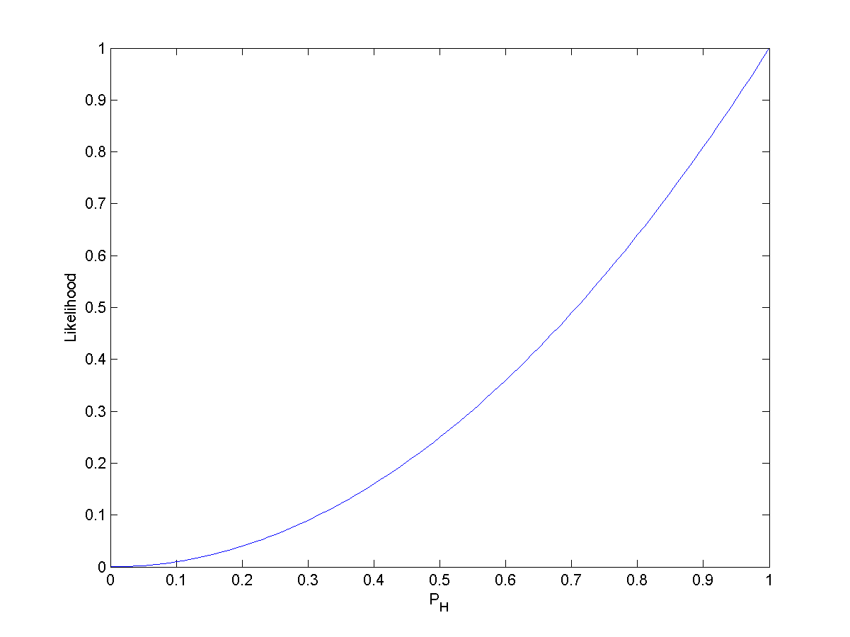
The likelihood function for estimating the probability of a coin landing heads-up without prior knowledge after observing HH

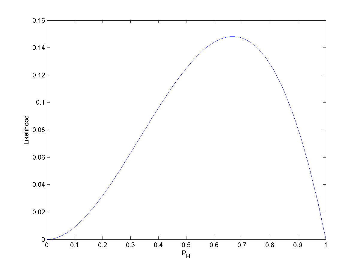
The likelihood function for estimating the probability of a coin landing heads-up without prior knowledge after observing HHT

Let p_H be the probability that a certain coin lands heads up (H) when tossed. So, the probability of getting two heads in two tosses (HH) is $p_\text{H}^2$. If p_H = 0.5, then the probability of seeing two heads is 0.25.

In symbols, we can say the above as:

P(HH | p_H = 0.5) = 0.25.

Another way of saying this is to reverse it and say that "the likelihood that p_H = 0.5, given the observation HH, is 0.25"; that is:

$\mathcal{L}(p_\text{H}=0.5 | \text{HH}) = P(\text{HH} | p_\text{H}=0.5) = 0.25.$

But this is not the same as saying that the probability that p_H = 0.5, given the observation HH, is 0.25.

Notice that the likelihood that p_H = 1, given the observation HH, is 1. But it is clearly not true that the probability that p_H = 1, given the observation HH, is 1. Two heads in a row hardly proves that the coin always comes up heads. In fact, two heads in a row is possible for any p_H > 0.

The likelihood function is not a probability density function. Notice that the integral of a likelihood function is not in general 1. In this example, the integral of the likelihood over the interval [0, 1] in p_H is 1/3, demonstrating that the likelihood function cannot be interpreted as a probability density function for p_H.

Example 2

Main article: German tank problem

Consider a jar containing N lottery tickets numbered from 1 through N. If you pick a ticket randomly then you get positive integer n, with probability 1/N if n ≤ N and with probability zero if n > N. This can be written

$P(n|N)= \frac{[n \le N]}{N}$

where the Iverson bracket [n ≤ N] is 1 when n ≤ N and 0 otherwise. When considered a function of n for fixed N this is the probability distribution, but when considered a function of N for fixed n this is a likelihood function. The maximum likelihood estimate for N is N₀ = n (by contrast, the unbiased estimate is 2n − 1).

This likelihood function is not a probability distribution, because the total

$\sum_{N=1}^\infty P(n|N) = \sum_{N} \frac{[N \ge n]}{N} = \sum_{N=n}^\infty \frac{1}{N}$

is a divergent series.

Suppose, however, that you pick two tickets rather than one.

The probability of the outcome {n₁, n₂}, where n₁ < n₂, is

$P(\{n_1,n_2\}|N)= \frac{[n_2 \le N]}{\binom N 2} .$

When considered a function of N for fixed n₂, this is a likelihood function. The maximum likelihood estimate for N is N₀ = n₂.

This time the total

$\sum_{N=1}^\infty P(\{n_1,n_2\}|N) = \sum_{N} \frac{[N\ge n_2]}{\binom N 2} =\frac 2 {n_2-1}$

is a convergent series, and so this likelihood function can be normalized into a probability distribution.

If you pick 3 or more tickets, the likelihood function has a well defined mean value, which is larger than the maximum likelihood estimate. If you pick 4 or more tickets, the likelihood function has a well defined standard deviation too.

Relative likelihood

Relative likelihood function

Suppose that the maximum likelihood estimate for θ is $\hat \theta$. Relative plausibilities of other θ values may be found by comparing the likelihood of those other values with the likelihood of $\hat \theta$. The relative likelihood of θ is defined^[2] as $\mathcal{L}(\theta | x)/\mathcal{L}(\hat \theta | x)$.

A 10% likelihood region for θ is

$\{\theta : \mathcal{L}(\theta | x)/\mathcal{L}(\hat \theta | x) \ge 0.10\},$

and more generally, a p% likelihood region for θ is defined^[2] to be

$\{\theta : \mathcal{L}(\theta | x)/\mathcal{L}(\hat \theta | x) \ge p/100 \}.$

If θ is a single real parameter, a p% likelihood region will typically comprise an interval of real values. In that case, the region is called a likelihood interval.^[2][3]

Likelihood intervals can be compared to confidence intervals. If θ is a single real parameter, then under certain conditions, a 14.7% likelihood interval for θ will be the same as a 95% confidence interval.^[2] In a slightly different formulation suited to the use of log-likelihoods, the e⁻² likelihood interval is the same as the 0.954 confidence interval (under certain conditions).^[3]

The idea of basing an interval estimate on the relative likelihood goes back to Fisher in 1956 and has been by many authors since then.^[3] If a likelihood interval is specifically to be interpreted as a confidence interval, then this idea is immediately related to the likelihood ratio test which can be used to define appropriate intervals for parameters. This approach can be used to define the critical points for the likelihood ratio statistic to achieve the required coverage level for a confidence interval. However a likelihood interval can be used as such, having been determined in a well-defined way, without claiming any particular coverage probability.

Relative likelihood of models

The definition of relative likelihood can also be generalized to compare different (fitted) statistical models. This generalization is based on Akaike information criterion, or more usually, AICc (Akaike Information Criterion with correction). Suppose that, for some dataset, we have two statistical models, M₁ and M₂, with fixed parameters. Also suppose that AICc(M₁) ≤ AICc(M₂). Then the relative likelihood of M₂ with respect to M₁ is defined^[4] to be

exp((AICc(M₁)−AICc(M₂))/2)

To see that this is a generalization of the earlier definition, suppose that we have some model M with a (possibly multivariate) parameter θ. Then for any θ, set M₂ = M(θ), and also set M₁ = M($\hat\theta$). The general definition now gives the same result as the earlier definition.^{[clarification needed]}

Likelihoods that eliminate nuisance parameters

In many cases, the likelihood is a function of more than one parameter but interest focuses on the estimation of only one, or at most a few of them, with the others being considered as nuisance parameters. Several alternative approaches have been developed to eliminate such nuisance parameters so that a likelihood can be written as a function of only the parameter (or parameters) of interest; the main approaches being marginal, conditional and profile likelihoods.^[5][6]

These approaches are useful because standard likelihood methods can become unreliable or fail entirely when there are many nuisance parameters or when the nuisance parameters are high-dimensional. This is particularly true when the nuisance parameters can be considered to be "missing data"; they represent a non-negligible fraction of the number of observations and this fraction does not decrease when the sample size increases. Often these approaches can be used to derive closed-form formulae for statistical tests when direct use of maximum likelihood requires iterative numerical methods. These approaches find application in some specialized topics such as sequential analysis.

Conditional likelihood

Sometimes it is possible to find a sufficient statistic for the nuisance parameters, and conditioning on this statistic results in a likelihood which does not depend on the nuisance parameters.

One example occurs in 2×2 tables, where conditioning on all four marginal totals leads to a conditional likelihood based on the non-central hypergeometric distribution. This form of conditioning is also the basis for Fisher's exact test.

Marginal likelihood

Main article: Marginal likelihood

Sometimes we can remove the nuisance parameters by considering a likelihood based on only part of the information in the data, for example by using the set of ranks rather than the numerical values. Another example occurs in linear mixed models, where considering a likelihood for the residuals only after fitting the fixed effects leads to residual maximum likelihood estimation of the variance components.

Profile likelihood

It is often possible to write some parameters as functions of other parameters, thereby reducing the number of independent parameters. (The function is the parameter value which maximizes the likelihood given the value of the other parameters.) This procedure is called concentration of the parameters and results in the concentrated likelihood function, also occasionally known as the maximized likelihood function, but most often called the profile likelihood function.

For example, consider a regression analysis model with normally distributed errors. The most likely value of the error variance is the variance of the residuals. The residuals depend on all other parameters. Hence the variance parameter can be written as a function of the other parameters.

Unlike conditional and marginal likelihoods, profile likelihood methods can always be used, even when the profile likelihood cannot be written down explicitly. However, the profile likelihood is not a true likelihood, as it is not based directly on a probability distribution, and this leads to some less satisfactory properties. Attempts have been made to improve this, resulting in modified profile likelihood.

The idea of profile likelihood can also be used to compute confidence intervals that often have better small-sample properties than those based on asymptotic standard errors calculated from the full likelihood. In the case of parameter estimation in partially observed systems, the profile likelihood can be also used for identifiability analysis.^[7] An implementation is available in the MATLAB Toolbox PottersWheel.

Partial likelihood

A partial likelihood is a factor component of the likelihood function that isolates the parameters of interest.^[8] It is a key component of the proportional hazards model.

Historical remarks

In English, "likelihood" has been distinguished as being related to but weaker than "probability" since its earliest uses. The comparison of hypotheses by evaluating likelihoods has been used for centuries, for example by John Milton in Aeropagitica: "when greatest likelihoods are brought that such things are truly and really in those persons to whom they are ascribed".

In Danish, "likelihood" was used by Thorvald N. Thiele in 1889.^[9][10][11]

In English, "likelihood" appears in many writings by Charles Sanders Peirce, where model-based inference (usually abduction but sometimes including induction) is distinguished from statistical procedures based on objective randomization. Peirce's preference for randomization-based inference is discussed in "Illustrations of the Logic of Science" (1877–1878) and "A Theory of Probable Inference" (1883)".

"probabilities that are strictly objective and at the same time very great, although they can never be absolutely conclusive, ought nevertheless to influence our preference for one hypothesis over another; but slight probabilities, even if objective, are not worth consideration; and merely subjective likelihoods should be disregarded altogether. For they are merely expressions of our preconceived notions" (7.227 in his Collected Papers).

"But experience must be our chart in economical navigation; and experience shows that likelihoods are treacherous guides. Nothing has caused so much waste of time and means, in all sorts of researchers, as inquirers' becoming so wedded to certain likelihoods as to forget all the other factors of the economy of research; so that, unless it be very solidly grounded, likelihood is far better disregarded, or nearly so; and even when it seems solidly grounded, it should be proceeded upon with a cautious tread, with an eye to other considerations, and recollection of the disasters caused." (Essential Peirce, volume 2, pages 108–109)

Like Thiele, Peirce considers the likelihood for a binomial distribution. Peirce uses the logarithm of the odds-ratio throughout his career. Peirce's propensity for using the log odds is discussed by Stephen Stigler.^{[citation needed]}

In Great Britain, "likelihood" was popularized in mathematical statistics by R.A. Fisher in 1922^[12]: "On the mathematical foundations of theoretical statistics". In that paper, Fisher also uses the term "method of maximum likelihood". Fisher argues against inverse probability as a basis for statistical inferences, and instead proposes inferences based on likelihood functions. Fisher's use of "likelihood" fixed the terminology that is used by statisticians throughout the world.

See also

• Bayes factor
• Bayesian inference
• Conditional probability
• Likelihood principle
• Maximum likelihood
• Likelihood-ratio test
• Principle of maximum entropy
• Conditional entropy
• Score (statistics)

Notes

1. ^ Edwards, A.W.F. 1972. Likelihood. Cambridge University Press, Cambridge (expanded edition, 1992, Johns Hopkins University Press, Baltimore). ISBN 0-8018-4443-6
2. ^ ^{a b c d} Kalbfleisch J.G. (1985) Probability and Statistical Inference, Springer (§9.3.)
3. ^ ^{a b c} Hudson, D. J. (1971). "Interval Estimation from the Likelihood Function". Journal of the Royal Statistical Society, Series B 33 (2): 256–262. 
4. ^ Burnham K. P. & Anderson D.R. (2002), Model Selection and Multimodel Inference, §2.8 (Springer).
5. ^ Pawitan, Yudi (2001). In All Likelihood: Statistical Modelling and Inference Using Likelihood. Oxford University Press. ISBN 0198507658. 
6. ^ Wen Hsiang Wei. "Generalized linear model course notes". Tung Hai University, Taichung, Taiwan. pp. Chapter 5. http://web.thu.edu.tw/wenwei/www/glmpdfmargin.htm. Retrieved 2007-01-23. 
7. ^ Raue, A; Kreutz, C; Maiwald, T; Bachmann, J; Schilling, M; Klingmüller, U; Timmer, J (2009). "Structural and practical identifiability analysis of partially observed dynamical models by exploiting the profile likelihood". Bioinformatics 25 (15): 1923–9. doi:10.1093/bioinformatics/btp358. PMID 19505944. http://bioinformatics.oxfordjournals.org/cgi/content/abstract/btp358?ijkey=iYp4jPP50F5vdX0&keytype=ref. 
8. ^ Cox, D. R. (1975). "Partial likelihood". Biometrika 62 (2): 269–276. doi:10.1093/biomet/62.2.269. MR0400509. 
9. ^ Anders Hald (1998). A History of Mathematical Statistics from 1750 to 1930. New York: Wiley. ISBN 0471179124. 
10. ^ Steffen L. Lauritzen, Aspects of T. N. Thiele’s Contributions to Statistics. Bulletin of the International Statistical Institute, 58, 27–30, 1999.
11. ^ Steffen L. Lauritzen (2002). Thiele: Pioneer in Statistics. [Oxford University Press]. pp. 288. ISBN 978-0-19-850972-1. 
12. ^ Fisher, R.A. (1922). "On the mathematical foundations of theoretical statistics". Philosophical Transactions of the Royal Society of London. Series A 222 (594–604): 309–368. doi:10.1098/rsta.1922.0009. JFM 48.1280.02. JSTOR 91208. http://digital.library.adelaide.edu.au/dspace/handle/2440/15172. 

References

• John W. Pratt (May 1976). "F. Y. Edgeworth and R. A. Fisher on the Efficiency of Maximum Likelihood Estimation". The Annals of Statistics 4 (3): 501–514. doi:10.1214/aos/1176343457.  | jstor = 2958222
• Stephen M. Stigler (1978). "Francis Ysidro Edgeworth, Statistician". Journal of the Royal Statistical Society, Series A 141 (3): 287–322. doi:10.2307/2344804. JSTOR 2344804.  | jstor = 2344804
• Stephen M. Stigler. The History of Statistics: The Measurement of Uncertainty before 1900. Harvard University Press. ISBN 0-674-40340-1. 
• Stephen M. Stigler. Statistics on the Table: The History of Statistical Concepts and Methods. Harvard University Press. ISBN 0-674-83601-4. 
• Anders Hald (1999). "On the History of Maximum Likelihood in Relation to Inverse Probability and Least Squares". Statistical Science 14 (2): 214–222.  | jstor = 2676741
• Hald, A. (1998). A History of Mathematical Statistics from 1750 to 1930. New York: Wiley. ISBN 0471179124. 

External links

• Likelihood function at Planetmath