German tank problem

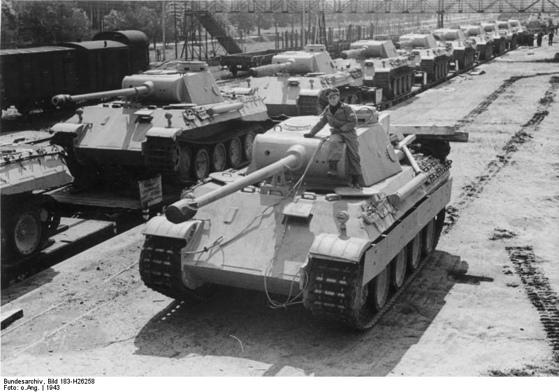
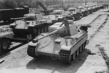During World War II, production of German tanks such as the Panther was accurately estimated by Allied intelligence using statistical methods.

In the statistical theory of estimation, estimating the maximum of a uniform distribution is a common illustration of differences between estimation methods. The specific case of sampling without replacement from a discrete uniform distribution is known, in the English-speaking world, as the German tank problem, due to its application in World War II to the estimation of the number of German tanks.

Estimating the population maximum based on a single sample yields divergent results, while the estimation based on multiple samples is an instructive practical estimation question whose answer is simple but not obvious.

Historical problem

In wartime, a key goal of military intelligence is to determine the strength of an enemy force: in World War II, the Western Allies wanted to estimate the number of tanks the Germans had, and approached this in two major ways: conventional intelligence gathering, and statistical estimation. The statistical approach proved to be far more accurate than conventional intelligence methods; the primary reference for the statistical approach is Ruggles & Brodie (1947).^{[1][notes 1]} In some cases statistical analysis contradicted and substantially improved on conventional intelligence; in others, conventional intelligence and the statistical approach worked together, as in estimation of Panther tank production, discussed below. Estimating production was not the only use of this serial number analysis; it was used to understand German production more generally, including number of factories, relative importance of factories, length of supply chain (based on lag between production and use), changes in production, and use of resources such as rubber.

To estimate the number of tanks produced up to a certain point, the Allies used the serial numbers on tanks. The principal numbers used were gearbox numbers, as these fell in two unbroken sequences. Chassis and engine numbers were also used, though their use were more complicated – various other components were used in the cross-checking of the analysis. Similar analyses were done on tires.^[1] which were observed to be sequentially numbered (i.e. 1, 2, 3, ..., N).^{[notes 2][2][3]}

Specific data

According to conventional Allied intelligence estimates the Germans were producing around 1,400 tanks a month between June 1940 and September 1942. Applying the above formula to the serial numbers of captured German tanks, (both serviceable and destroyed) the number was calculated to be 256 a month. After the war, captured German production figures from the ministry of Albert Speer showed the actual number to be 255.^[2]

Estimates for some specific months is given as:^[4][5]

Month	Statistical estimate	Intelligence estimate	German records
June 1940	169	1000	122
June 1941	244	1550	271
August 1942	327	1550	342

Shortly before D-Day, following rumors of large Panther tank production collected by conventional intelligence, analysis of road wheels from two tanks (consisting of 48 wheels each, for 96 wheels total) yielded an estimate of 270 Panthers produced in February 1944, substantially more than had previously been suspected; German records after the war showed production for that month was 276.^[6] Specifically, analysis of the wheels yielded an estimate for the number of wheel molds; discussion with British road wheel makers then estimated the number of wheels that could be produced from this many molds.

Similar analyses

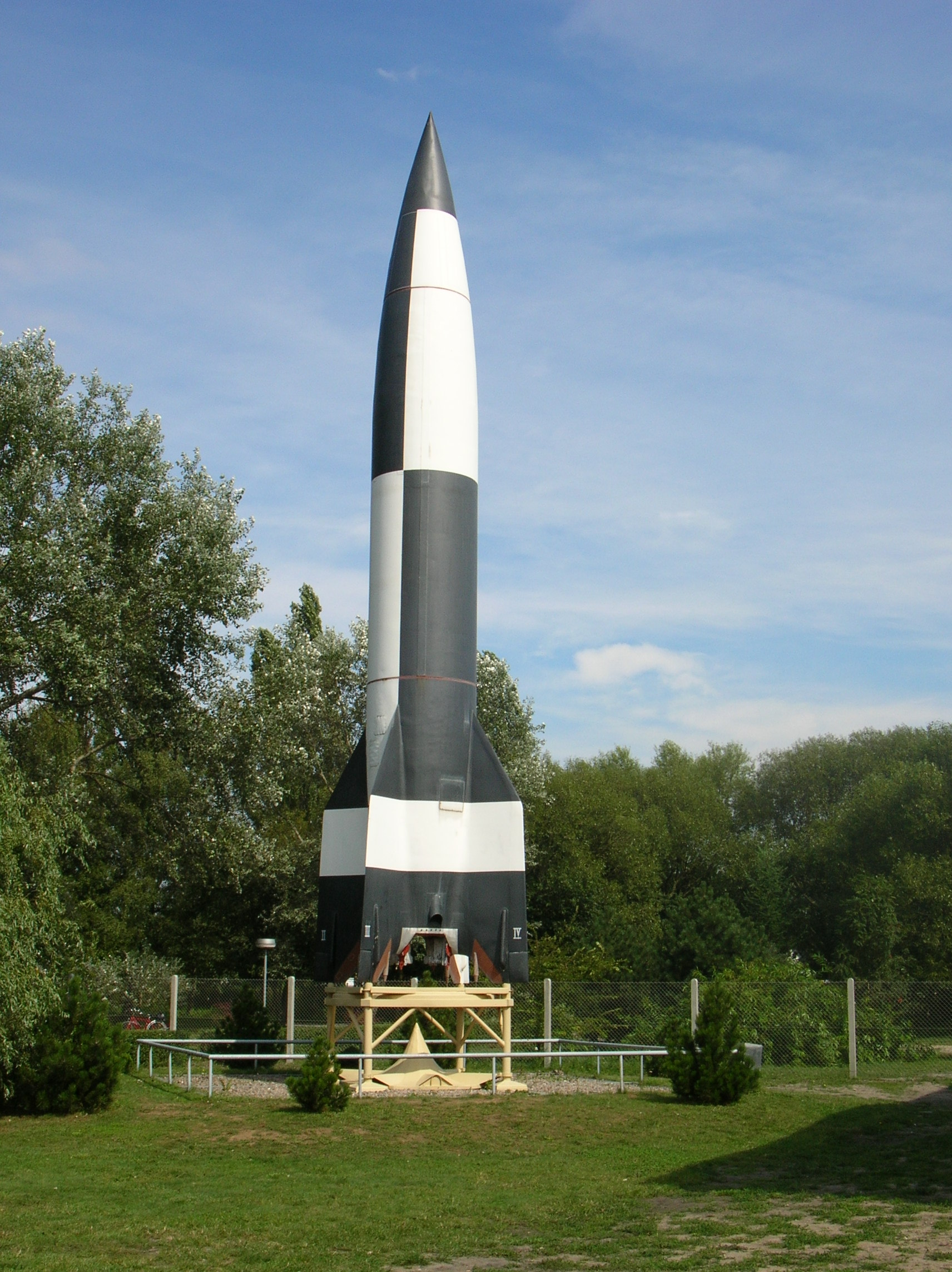
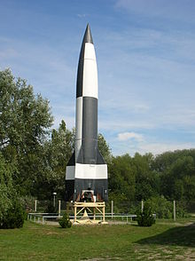V-2 rocket production was accurately estimated by statistical methods.

Similar serial number analysis was used for other military equipment during World War II, most successfully for the V-2 rocket.^[7]

During World War II, German intelligence analyzed factory markings on Soviet military equipment, and during the Korean war, factory markings on Soviet equipment was again analyzed. The Soviets also estimated German tank production during World War II.^[8]

In the 1980s, some Americans were given access to the production line of Israel’s Merkava tanks. The production numbers were classified, but the tanks had serial numbers, allowing estimation of production.^[9]

Countermeasures

To prevent serial number analysis, one can most simply not include serial numbers, or reduce auxiliary information that can be usable. Alternatively, one can design serial numbers that resist cryptanalysis, most effectively by randomly choosing numbers without replacement from a list that is much larger than the number of objects you produce (compare the one-time pad), or simply produce random numbers and check them against the list of already assigned numbers; collisions are likely to occur unless the number of digits possible is more than twice as many as the number of digits in the number of objects produced (where the serial number can be in decimal, hexadecimal or indeed in any base); see birthday problem.^{[notes 3]} For this, one may use a cryptographically secure pseudorandom number generator. Less securely, to avoid lookup problems, one may use any pseudorandom number generator with large period, which is guaranteed to avoid collisions. All these methods require a lookup table (or breaking the cypher) to back out from serial number to production order, which complicates use of serial numbers: one cannot simply recall a range of serial numbers, for instance, but instead must look them each up individually, or generate a list.

Alternatively, one can simply use sequential serial numbers and encrypt them, which allows easy decoding, but then there is a known-plaintext attack: even if one starts from an arbitrary point, the plaintext has a pattern (namely, numbers are in sequence).

Frequentist analysis

Minimum-variance unbiased estimator

For point estimation (estimating a single value for the total), the minimum-variance unbiased estimator (MVUE, or UMVU estimator) is given by:^{[notes 4]}

$\hat{N} =m(1 + k^{-1}) - 1\,$

where m is the largest serial number observed (sample maximum) and k is the number of tanks observed (sample size).^[9][10][11] Note that once a serial number has been observed, it is no longer in the pool and will not be observed again.

This has a variance of^[9]

$\operatorname{var}(\hat{N}) = \frac{1}{k}\frac{(N-k)(N+1)}{(k+2)} \approx \frac{N^2}{k^2} \text{ for small samples } k \ll N$

so a standard deviation of approximately N/k, the (population) average size of a gap between samples; compare m/k above.

Example

Suppose there are 15 tanks, numbered 1, 2, 3, ..., 15. An intelligence officer has spotted tanks 2, 6, 7, 14. Using the above formula, the values for m and k would be 14 and 4, respectively. The formula m(1 + k ^{− 1}) − 1 gives a value 16.5, which is close to the actual number of tanks, 15. Then suppose the officer spots an additional 2 tanks, neither of them #15. Now k = 6 and m remains 14. The formula gives a better estimate of 15.333...

Intuition

The formula may be understood intuitively as:

"The sample maximum plus the average gap between observations in the sample",

the gap being added to compensate for the negative bias of the sample maximum as an estimator for the population maximum,^{[notes 5]} and written as

$\hat{N}= m + \frac{m-k}{k}= m + \frac\text{missing numbers}{k}.$

This can be visualized by imagining that the samples are evenly spaced throughout the range, with additional samples just outside the range at 0 and N + 1. If one starts with an initial gap being between 0 and the lowest sample (sample minimum), then the average gap between samples is m/k − 1; the −1 being because one does not count the samples themselves in computing the gap between samples.^{[notes 6]}

This philosophy is formalized and generalized in the method of maximum spacing estimation.

Derivation

The probability that the sample maximum equals m is $\frac{\tbinom{m-1}{k-1}}{\tbinom Nk}$, where $\tbinom \cdot\cdot$ is the binomial coefficient.

The expected value of the sample maximum is

$\mu=\sum_{m=k}^N m\frac{\tbinom{m-1}{k-1}}{\tbinom Nk} = \frac{k(N+1)}{k+1}$

Solving for N gives $N=\mu(1+k^{-1})-1\,.$

Since $\mu(1+k^{-1})-1=E(m(1+k^{-1})-1)\,$ it follows that

$\hat{N} =m(1 + k^{-1}) - 1\,$

is an unbiased estimator of N.

To show that this is the UMVU estimator:

• One first shows that the sample maximum is a sufficient statistic for the population maximum, using a method similar to that detailed at sufficiency: uniform distribution (but for the German tank problem we must exclude the outcomes in which a serial number occurs twice in the sample);
• Next, one shows that it is a complete statistic.
• Then the Lehmann–Scheffé theorem states that the sample maximum, corrected for bias as above to be unbiased, is the UMVU estimator.

Confidence intervals

Instead of, or in addition to, point estimation, one can do interval estimation, such as confidence intervals. These are easily computed, based on the observation that the odds that k samples will fall in an interval covering p of the range (0 ≤ p ≤ 1) is p^k (assuming in this section that draws are with replacement, to simplify computations; if draws are without replacement, this overstates the likelihood, and intervals will be overly conservative).

Thus the sampling distribution of the quantile of the sample maximum is the graph x^1/k from 0 to 1: the pth to qth quantile of the sample maximum m are the interval [p^1/kN, q^1/kN]. Inverting this yields the corresponding confidence interval for the population maximum of [m/q^1/k, m/p^1/k].

For example, taking the symmetric 95% interval p = 2.5% and q = 97.5% for k = 5 yields $0.025^{1/5} \approx 0.48, 0.975^{1/5} \approx 0.995$, so a confidence interval of approximately [1.005m,2.08m]. The lower bound is very close to m, so more informative is the asymmetric confidence interval from p = 5% to 100%; for k = 5 this yields $0.05^{1/5} \approx 0.55,$ so the interval [m, 1.82m].

More generally, the (downward biased) 95% confidence interval is $[m,m/.05^{1/k}]=[m,m\cdot 20^{1/k}].$ For a range of k, with the UMVU point estimator (plus 1 for legibility) for reference, this yields:

k	point estimate	confidence interval
1	2m	[m,20m]
2	1.5m	[m,4.5m]
5	1.2m	[m,1.82m]
10	1.1m	[m,1.35m]
20	1.05m	[m,1.16m]

Immediate observations are:

• For small sample sizes, the confidence interval is very wide, reflecting great uncertainty in the estimate.
• The range shrinks rapidly, reflecting the exponentially decaying likelihood that all samples will be significantly below the maximum.
• The confidence interval exhibits positive skew, as N can never be below the sample maximum, but can potentially be arbitrarily high above it.

Note that one cannot naively use m/k (or rather (m + m/k − 1)/k) as an estimate of the standard error SE, as the standard error of an estimator is based on the population maximum (a parameter), and using an estimate to estimate the error in that very estimate is circular reasoning.

Bayesian analysis

Summary

The Bayesian inference approach to the German Tank Problem is to consider the conditional probability Pr(N | m,k) that the number of enemy tanks is equal to N, when k serial numbers have been observed, and the largest of these is m.

$\Pr(N|m,k)=\Pr(m|N,k)\frac {\Pr(N)}{\Pr(m)}$

Then

$\Pr(N|m,k) =\frac{\Pr(N|m,k)}1 =\frac{\Pr(m|N,k)\frac {\Pr(N)}{\Pr(m)}}{\sum_{N=0}^\infty \Pr(m|N,k)\frac {\Pr(N)}{\Pr(m)}} =\frac{\Pr(m|N,k)\Pr(N)}{\sum_{N=0}^\infty \Pr(m|N,k)\Pr(N)}$

Assume that the prior probability Pr(N) is some discrete uniform distribution $\frac{[N<\Omega]}{\Omega}$, (where the Iverson bracket [N < Ω] means 1 when N < Ω and 0 otherwise). The upper limit Ω must be finite, because $\lim_{\Omega\rarr\infty}\frac{[N<\Omega]}{\Omega}$ is not a probability mass function of N.

Then

$\Pr(N|m,k)=\frac{\Pr(m|N,k)[N<\Omega]}{\sum_{N=m}^{\Omega-1} \Pr(m|N,k)}\approx\frac{\Pr(m|N,k)}{\sum_{N=m}^\infty \Pr(m|N,k)}$

If ${\sum_{N=m}^\infty \Pr(m|N,k)}<\infty$, then the approximation is adequate, and the unwelcome variable Ω vanishes from the expressions.

The conditional probability that the largest tank number observed is equal to m, when the number of enemy tanks is equal to N, and k enemy tanks has been observed, is

$\Pr(m|N,k)=\frac{\binom{m-1}{k-1}}{\binom{N}{k}}[m \le N]$

where the binomial coefficient $\scriptstyle \binom N k$ is the number of k-sized samples from an N-sized population.

For k≥1 the mode of the distribution of the number of enemy tanks is m.

For k≥2, the probability that the number of enemy tanks is equal to N, is $\Pr(N|m,k)\approx(1-k^{-1})\frac {\binom{m-1}{k-1}}{\binom N k}[N\ge m]$, and the probability that the number of enemy tanks is greater than N, is $\frac{\binom{m-1}{k-1}}{\binom{N}{k-1}}[N\ge m]$.

For k≥3, N has the finite mean value $\frac{(m-1)(k-1)}{k-2}$.

For k≥4, N has the finite standard deviation $\sqrt{\frac{(m-1)(k-1)(m+1-k)}{(k-2)^2(k-3)}}$

If tank numbers 2, 6, 7, and 14 were identified, then the posterior probability mass function is $\frac{5148[N\ge 14]}{N(N-1)(N-2)(N-3)}$. The mean value of N is 19.5 and the standard deviation of N is 10.4, so we estimate that the enemy has got 20 tanks, give or take 10. Of course we still know that they have got at least 14 tanks. The distribution has positive skewness.

The following important formula 14 from Binomial coefficient#Identities involving binomial coefficients is used below for simplifying series relating to the German Tank Problem.

$\sum_{N=m}^\infty \frac 1 {\binom N k}=\frac k{(k-1)\binom{m-1}{k-1}}$

One tank

If you observe one tank randomly out of a population of N tanks, you get serial number m with probability 1/N for m ≤ N, and zero probability for m > N. This is written

$\Pr(m|N) = \frac{[m \le N]}{N}$

This is the conditional probability mass function of m.

When considered a function of N for fixed m this is a likelihood function.

$\mathcal{L}(N) =\Pr(m|N) = \frac{[N \ge m]}N$.

The maximum likelihood estimate for N is N₀ = m.

The total likelihood is a infinite, being a tail of the harmonic series.

$\sum_N \mathcal{L}(N) =\sum_{N=m}^\infty \frac 1 N = \infty \,$

but

$\sum_N \mathcal{L}(N)[N<\Omega]=\sum_{N=m}^{\Omega-1} \frac 1 N = H_{\Omega-1}-H_{m-1}$

where H_n is the harmonic number.

The probability mass function of N depends explicitly on the prior limit Ω:

$\Pr(N|m)=\frac{[m \le N]}{N}\frac{[N< \Omega]}{H_{\Omega-1}-H_{m-1}}$.

The mean value of N is

$\sum_N N \Pr(N|m)=\sum_{N=m}^{\Omega-1} \frac{1}{H_{\Omega-1}-H_{m-1}}=\frac{\Omega-m}{H_{\Omega-1}-H_{m-1}}\approx \frac{\Omega}{\log(\frac{\Omega-1}{m-1})}.$

Two tanks

If you observe two tanks rather than one, then the probability that the larger of the observed two serial numbers is equal to m, is

$\Pr(m|N)= \frac{(m-1)[m\le N]}{\binom{N}{2}} .$

When considered a function of N for fixed m this is a likelihood function

$\mathcal{L}(N)=\frac{(m-1)[N \ge m]}{\binom{N}{2}} .$

The total likelihood is

$\sum_{N}\mathcal{L}(N)=(m-1)\sum_{N=m}^\infty {1\over \binom N 2}=2$.

and the probability mass function is

$\Pr(N|m)=\frac{\mathcal{L}(N)}{\sum_N \mathcal{L}(N)}=\frac{(m-1)[N\ge m]}{N(N-1)}$

The median $\tilde N$ satisfies

$\sum_N [N \ge \tilde N]P(N|m)=\frac 1 2$

so

$\frac {m-1} {\tilde N-1}=\frac 1 2$

and so the median is

$\tilde N=2m-1$

but the mean value of N is infinite

$\mu=\sum_N N\cdot \Pr(N|m)=(m-1)\sum_{N=m}^\infty \frac{1}{N-1}=\infty$

Many tanks

The conditional probability that the largest of k observations taken from the serial numbers {1,...,N}, is equal to m, is

$\Pr(m|N,k)=\frac{\binom{m-1}{k-1}[m \le N]}{\binom{N}{k}}.$

The likelihood function of N is the same expression

$\mathcal{L}(N)=\frac{\binom{m-1}{k-1}[N \ge m]}{\binom{N}{k}}.$

The total likelihood is finite for k ≥ 2:

$\sum_N \mathcal{L}(N)=\binom{m-1}{k-1}\sum_{N=m}^\infty {1\over \binom N k}=\frac k{k-1}$

The probability mass function of N is the probability that the number of enemy tanks is = N

$=\Pr(N|m,k)=\frac{\mathcal{L}(N)}{\sum_N \mathcal{L}(N)}=\frac {(k-1)\binom{m-1}{k-1}[N\ge m]}{k\binom N k}=\frac {(m-1)\binom{m-2}{k-2}[N\ge m]}{N\binom{N-1}{k-1}}$

The cumulative distribution function of N is the probability that the number of enemy tanks is ≤ N

$=\sum_{i=m}^N \frac {(m-1)\binom{m-2}{k-2}}{i\binom{i-1}{k-1}}=\left(1-\frac{\binom{m-1}{k-1}}{\binom{N}{k-1}}\right)[N\ge m]$

The expected number of enemy tanks is

$\mu =\sum_N N\cdot \Pr(N|m,k) =(m-1)\binom{m-2}{k-2}\sum_{N=m}^\infty \frac {1}{\binom{N-1}{k-1}} =\frac{(m-1)(k-1)}{k-2}$

The variance to mean ratio is computed like this.

$\begin{align} \frac{\sigma^2}{\mu} &=\frac{\sum_N N^2 \Pr(N|m,k) -\mu^2}{\mu} \\& =-\mu+\frac{\sum_N (N(N-1)+N)\Pr(N|m,k)}{\mu} \\& =-\mu+\frac{\sum_N N(N-1)\Pr(N|m,k)+\mu}{\mu} \\& =1-\mu+\sum_{N=m}^\infty \frac{(N-1)(m-1)\binom{m-2}{k-2}}{\mu \binom{N-1}{k-1}} \\& =1-\mu+\frac{(k-1)(m-1)\binom{m-2}{k-2}}{\mu}\sum_{N=m}^\infty \frac{1}{\binom{N-2}{k-2}} \\& =1-\mu+\frac{(k-1)(m-1)\frac{m-2}{k-2}\binom{m-3}{k-3}}{\mu} \frac{k-2}{(k-3)\binom{m-3}{k-3}} \\& =1-\frac{(m-1)(k-1)}{k-2}+\frac{(k-1)(m-1)(m-2)}{\frac{(m-1)(k-1)}{k-2}(k-3)} \\& =\frac{m+1-k}{(k-3)(k-2)} \end{align}$

and the standard deviation is

$\sigma=\sqrt{\mu\frac{m+1-k}{(k-3)(k-2)}}$

See also

• Capture-recapture, other method of estimating population size
• Maximum spacing estimation, which generalizes the intuition of "assume uniformly distributed"

Other discussions of the estimation

• Maximum likelihood#Bias
• Bias of an estimator#Maximum of a discrete uniform distribution
• Likelihood function#Example 5

Notes

1. ^ Ruggles & Brodie is largely a practical analysis and summary, not a mathematical one – the estimation problem is only mentioned in footnote 3 on page 82, where they estimate the maximum as "sample maximum + average gap".
2. ^ The lower bound was unknown, but to simplify the discussion this detail is generally omitted, taking the lower bound as known to be 1.
3. ^ As discussed in birthday attack, one can expect a collision after 1.25√H numbers, if choosing from H possible outputs. This square root corresponds to half the digits. For example, the square root of a number with 100 digits is approximately a number with 50 digits in any base.
4. ^ In a continuous distribution, there is no −1.
5. ^ The sample maximum is never more than the population maximum, but can be less, hence it is a biased estimator: it will tend to underestimate the population maximum.
6. ^ For example, the gap between 2 and 7 is (7 − 2) − 1 = 4, consisting of 3, 4, 5, and 6.

References

1. ^ ^{a b} Ruggles; Brodie, Henry (March 1947), "An empirical approach to economic intelligence in WWII", Journal of the American Statistical Association (American Statistical Association) 42 (237): 72–91, doi:10.2307/2280189, JSTOR 2280189 
2. ^ ^{a b} Gavyn Davies. How a statistical formula won the war The Guardian, 20 July 2006
3. ^ Matthews, Robert (1998-05-23), "Data sleuths go to war, sidebar in feature 'Hidden truths'", New Scientist, archived from the original on 2001-04-18, http://web.archive.org/web/20010418025817/http://www.newscientist.com/ns/980523/features.html#data 
4. ^ Ruggles & Brodie, p. 89
5. ^ Order Statistics, in Virtual Laboratories in Probability and Statistics
6. ^ Ruggles & Brodie, pp. 82–83
7. ^ Ruggles & Brodie, pp. 90–91
8. ^ Volz, Arthur G. (July 2008), "A Soviet Estimate of German Tank Production", The Journal of Slavic Military Studies 21 (3): 588–590, doi:10.1080/13518040802313902, http://www.informaworld.com/smpp/content~content=a901871255~db=all 
9. ^ ^{a b c} Johnson, Roger (1994), "Estimating the Size of a Population", Teaching Statistics 16 (2 (Summer)): 50, doi:10.1111/j.1467-9639.1994.tb00688.x 
10. ^ Johnson, Roger (2006), "Estimating the Size of a Population", Getting the Best from Teaching Statistics, http://www.rsscse.org.uk/ts/gtb/johnson.pdf 
11. ^ Joyce Smart. German Tank Problem Logan High School cites Activity Based Statistics [by Richard L. Schaeffer] p. 148-150. Exploring Surveys and Information from Samples, [by James M. Landwehr] Section IX, p. 75–83. Statistical Reasoning, Gary Smith, p. 148-149

General

• Goodman, L. A. (1954), "Some Practical Techniques in Serial Number Analysis", Journal of the American Statistical Association (American Statistical Association) 49 (265): 97–112, doi:10.2307/2281038, JSTOR 2281038