Maximum power transfer theorem

In electrical engineering, the maximum power transfer theorem states that, to obtain maximum external power from a source with a finite internal resistance, the resistance of the load must be equal to the resistance of the source as viewed from the output terminals. Moritz von Jacobi published the maximum power (transfer) theorem around 1840, which is also referred to as "Jacobi's law".^[1]

The theorem results in maximum power transfer, and not maximum efficiency. If the resistance of the load is made larger than the resistance of the source, then efficiency is higher, since a higher percentage of the source power is transferred to the load, but the magnitude of the load power is lower since the total circuit resistance goes up.

If the load resistance is smaller than the source resistance, then most of the power ends up being dissipated in the source, and although the total power dissipated is higher, due to a lower total resistance, it turns out that the amount dissipated in the load is reduced.

The theorem states how to choose (so as to maximize power transfer) the load resistance, once the source resistance is given, not the opposite. It does not say how to choose the source resistance, once the load resistance is given. Given a certain load resistance, the source resistance that maximizes power transfer is always zero, regardless of the value of the load resistance.

The theorem can be extended to AC circuits that include reactance, and states that maximum power transfer occurs when the load impedance is equal to the complex conjugate of the source impedance.

Maximizing power transfer versus power efficiency

The theorem was originally misunderstood (notably by Joule) to imply that a system consisting of an electric motor driven by a battery could not be more than 50% efficient since, when the impedances were matched, the power lost as heat in the battery would always be equal to the power delivered to the motor. In 1880 this assumption was shown to be false by either Edison or his colleague Francis Robbins Upton, who realized that maximum efficiency was not the same as maximum power transfer. To achieve maximum efficiency, the resistance of the source (whether a battery or a dynamo) could be made close to zero. Using this new understanding, they obtained an efficiency of about 90%, and proved that the electric motor was a practical alternative to the heat engine.

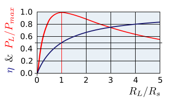
The condition of maximum power transfer does not result in maximum efficiency. If we define the efficiency η as the ratio of power dissipated by the load to power developed by the source, then it is straightforward to calculate from the above circuit diagram that

$\eta = {R_\mathrm{load} \over {R_\mathrm{load} + R_\mathrm{source} } } = { 1 \over { 1 + { R_\mathrm{source} \over R_\mathrm{load} } } }. \,\!$

Consider three particular cases:

• If $R_\mathrm{load}=R_\mathrm{source}\,\!$, then $\eta=0.5,\,\!$
• If $R_\mathrm{load}=\infty\,\!$ or $R_\mathrm{source} = 0,\,\!$ then $\eta=1,\,\!$
• If $R_\mathrm{load}=0\,\!$, then $\eta=0.\,\!$

The efficiency is only 50% when maximum power transfer is achieved, but approaches 100% as the load resistance approaches infinity, though the total power level tends towards zero. Efficiency also approaches 100% if the source resistance can be made close to zero. When the load resistance is zero, all the power is consumed inside the source (the power dissipated in a short circuit is zero) so the efficiency is zero.

Note that for a time varying voltage and current, the above applies only to the resistive component of the power, not the reactive component. As shown below, a proper pure reactive match can theoretically achieve 100% power transfer AND 100% efficiency simultaneously in a perfect resistance free reactive circuit. In an imperfect reactive circuit (i.e. one with both reactance and resistance), the efficiency will be the power dissipated in the load divided by the power provided by the source. When the resistance is a small fraction of the reactance, the efficiency will then be very high even at the maximum power transfer point. This is a key reason why power grids use AC versus DC power, and why radio frequency (RF) circuits can operate with relatively high efficiency.

Impedance matching

Main article: impedance matching

A related concept is reflectionless impedance matching. In radio, transmission lines, and other electronics, there is often a requirement to match the source impedance (such as a transmitter) to the load impedance (such as an antenna) to avoid reflections in the transmission line.

Calculus-based proof for purely resistive circuits

(See Cartwright^[2] for a non-calculus-based proof)

In the diagram opposite, power is being transferred from the source, with voltage $V \,\!$ and fixed source resistance $R_\mathrm{S} \,\!$, to a load with resistance $R_\mathrm{L} \,\!$, resulting in a current $I \,\!$. By Ohm's law, $I \,\!$ is simply the source voltage divided by the total circuit resistance:

$I = {V \over R_\mathrm{S} + R_\mathrm{L}}. \,\!$

The power $P_\mathrm{L} \,\!$ dissipated in the load is the square of the current multiplied by the resistance:

$P_\mathrm{L} = I^2 R_\mathrm{L} = {{ \left( {V \over {R_\mathrm{S} + R_\mathrm{L}}} \right) }^2} R_\mathrm{L} = {{V^2} \over {R_\mathrm{S}^2 / R_\mathrm{L} + 2R_\mathrm{S} + R_\mathrm{L}}}. \,\!$

The value of $R_\mathrm{L} \,\!$ for which this expression is a maximum could be calculated by differentiating it, but it is easier to calculate the value of $R_\mathrm{L} \,\!$ for which the denominator

$R_\mathrm{S}^2 / R_\mathrm{L} + 2R_\mathrm{S} + R_\mathrm{L} \,\!$

is a minimum. The result will be the same in either case. Differentiating the denominator with respect to $R_\mathrm{L} \,\!$:

${d\over{dR_\mathrm{L}}} \left( {R_\mathrm{S}^2 / R_\mathrm{L} + 2R_\mathrm{S} + R_\mathrm{L}} \right) = -R_\mathrm{S}^2 / R_\mathrm{L}^2+1. \,\!$

For a maximum or minimum, the first derivative is zero, so

${R_\mathrm{S}^2 / R_\mathrm{L}^2} = 1 \,\!$

or

$R_\mathrm{L} = \pm R_\mathrm{S}. \,\!$

In practical resistive circuits, $R_\mathrm{S} \,\!$ and $R_\mathrm{L} \,\!$ are both positive, so the positive sign in the above is the correct solution. To find out whether this solution is a minimum or a maximum, the denominator expression is differentiated again:

${{d^2} \over {dR_\mathrm{L}^2}} \left( {R_\mathrm{S}^2 / R_\mathrm{L} + 2 R_\mathrm{S} + R_\mathrm{L}} \right) = {2 R_\mathrm{S}^2} / {R_\mathrm{L}^3}. \,\!$

This is always positive for positive values of $R_\mathrm{S} \,\!$ and $R_\mathrm{L} \,\!$, showing that the denominator is a minimum, and the power is therefore a maximum, when

$R_\mathrm{S} = R_\mathrm{L}. \,\!$

A note of caution is in order here. This last statement, as written, implies to many people that for a given load, the source resistance must be set equal to the load resistance for maximum power transfer. However, this equation only applies if the source resistance cannot be adjusted, e.g., with antennas (see the first line in the proof stating "fixed source resistance"). For any given load resistance a source resistance of zero is the way to transfer maximum power to the load. As an example, a 100 volt source with an internal resistance of 10 ohms connected to a 10 ohm load will deliver 250 watts to that load. Make the source resistance zero ohms and the load power jumps to 1000 watts.

In reactive circuits

The theorem also applies where the source and/or load are not totally resistive. This invokes a refinement of the maximum power theorem, which says that any reactive components of source and load should be of equal magnitude but opposite phase. (See below for a derivation.) This means that the source and load impedances should be complex conjugates of each other. In the case of purely resistive circuits, the two concepts are identical. However, physically realizable sources and loads are not usually totally resistive, having some inductive or capacitive components, and so practical applications of this theorem, under the name of complex conjugate impedance matching, do, in fact, exist.

If the source is totally inductive (capacitive), then a totally capacitive (inductive) load, in the absence of resistive losses, would receive 100% of the energy from the source but send it back after a quarter cycle. The resultant circuit is nothing other than a resonant LC circuit in which the energy continues to oscillate to and fro. This is called reactive power. Power factor correction (where an inductive reactance is used to "balance out" a capacitive one), is essentially the same idea as complex conjugate impedance matching although it is done for entirely different reasons.

For a fixed reactive source, the maximum power theorem maximizes the real power (P) delivered to the load by complex conjugate matching the load to the source.

For a fixed reactive load, power factor correction minimizes the apparent power (S) (and unnecessary current) conducted by the transmission lines, while maintaining the same amount of real power transfer. This is done by adding a reactance to the load to balance out the load's own reactance, changing the reactive load impedance into a resistive load impedance.

Proof

In this diagram, AC power is being transferred from the source, with phasor magnitude voltage | V_S | (peak voltage) and fixed source impedance Z_S, to a load with impedance Z_L, resulting in a phasor magnitude current | I | . | I | is simply the source voltage divided by the total circuit impedance:

$|I| = { |V_\mathrm{S}| \over |Z_\mathrm{S} + Z_\mathrm{L}| }.$

The average power P_L dissipated in the load is the square of the current multiplied by the resistive portion (the real part) R_L of the load impedance:

$\begin{align} P_\mathrm{L} & = I_\mathrm{rms}^2 R_\mathrm{L} = {1 \over 2} |I|^2 R_\mathrm{L} = {1 \over 2} \left( {|V_\mathrm{S}| \over |Z_\mathrm{S} + Z_\mathrm{L}|} \right)^2 R_\mathrm{L} \\ & = {1 \over 2}{ |V_\mathrm{S}|^2 R_\mathrm{L} \over (R_\mathrm{S} + R_\mathrm{L})^2 + (X_\mathrm{S} + X_\mathrm{L})^2}, \end{align}$

where the resistance R_S and reactance X_S are the real and imaginary parts of Z_S, and X_L is the imaginary part of Z_L.

To determine the values of R_L and X_L (since V_S, R_S, and X_S are fixed) for which this expression is a maximum, we first find, for each fixed positive value of R_L, the value of the reactive term X_L for which the denominator

$(R_\mathrm{S} + R_\mathrm{L})^2 + (X_\mathrm{S} + X_\mathrm{L})^2 \,$

is a minimum. Since reactances can be negative, this denominator is easily minimized by making

$X_\mathrm{L} = -X_\mathrm{S}.\,$

The power equation is now reduced to:

$P_\mathrm{L} = {1 \over 2}{{|V_\mathrm{S}|^2 R_\mathrm{L}}\over{(R_\mathrm{S} + R_\mathrm{L})^2}}\,\!$

and it remains to find the value of R_L which maximizes this expression. However, this maximization problem has exactly the same form as in the purely resistive case, and the maximizing condition R_L = R_S can be found in the same way.

The combination of conditions

• $R_\mathrm{L} = R_\mathrm{S}\,\!$
• $X_\mathrm{L} = -X_\mathrm{S}\,\!$

can be concisely written with a complex conjugate (the *) as:

$Z_\mathrm{S} = Z_\mathrm{L}^*.$

See also

• Maximum power principle

Notes

1. ^ Thompson Phillips (2009-05-30), Dynamo-Electric Machinery; A Manual for Students of Electrotechnics, BiblioBazaar, LLC, ISBN 9781110351046, http://books.google.com/?id=dKVbT-ZmdDwC&pg=PA406 
2. ^ Cartwright, Kenneth V (Spring 2008), "Non-Calculus Derivation of the Maximum Power Transfer Theorem", Technology Interface 8 (2): 19 pages, http://technologyinterface.nmsu.edu/Spring08/ 

References

• H.W. Jackson (1959) Introduction to Electronic Circuits, Prentice-Hall.

External links

• The complex conjugate matching false idol
• Conjugate matching versus reflectionless matching (PDF) taken from Electromagnetic Waves and Antennas
• The Spark Transmitter. 2. Maximising Power, part 1.
• Jacobi's theorem - unconfirmed claim that theorem was discovered by Moritz Jacobi
• [1] MH Jacobi Biographical notes
• Google Docs Spreadsheet calculating max power transfer efficiencies by Sholto Maud and Dino Cevolatti.