Oblate spheroidal coordinates

Figure 1: Coordinate isosurfaces for a point P (shown as a black sphere) in oblate spheroidal coordinates (μ, ν, φ). The z-axis is vertical, and the foci are at ±2. The red oblate spheroid (flattened sphere) corresponds to μ=1, whereas the blue half-hyperboloid corresponds to ν=45°. The azimuth φ=-60° measures the dihedral angle between the green x-z half-plane and the yellow half-plane that includes the point P'. The Cartesian coordinates of P are roughly (1.09, -1.89, 1.66).

Oblate spheroidal coordinates are a three-dimensional orthogonal coordinate system that results from rotating the two-dimensional elliptic coordinate system about the non-focal axis of the ellipse, i.e., the symmetry axis that separates the foci. Thus, the two foci are transformed into a ring of radius a in the x-y plane. (Rotation about the other axis produces the prolate spheroidal coordinates.) Oblate spheroidal coordinates can also be considered as a limiting case of ellipsoidal coordinates in which the two largest semi-axes are equal in length.

Oblate spheroidal coordinates are often useful in solving partial differential equations when the boundary conditions are defined on an oblate spheroid or a hyperboloid of revolution. For example, they played an important role in the calculation of the Perrin friction factors, which contributed to the awarding of the 1926 Nobel Prize in Physics to Jean Baptiste Perrin. These friction factors determine the rotational diffusion of molecules, which affects the feasibility of many techniques such as protein NMR and from which the hydrodynamic volume and shape of molecules can be inferred. Oblate spheroidal coordinates are also useful in problems of electromagnetism (e.g., dielectric constant of charged oblate molecules), acoustics (e.g., scattering of sound through a circular hole), fluid dynamics (e.g., the flow of water through a firehose nozzle) and the diffusion of materials and heat (e.g., cooling of a red-hot coin in a water bath).

Definition (μ, ν, φ)

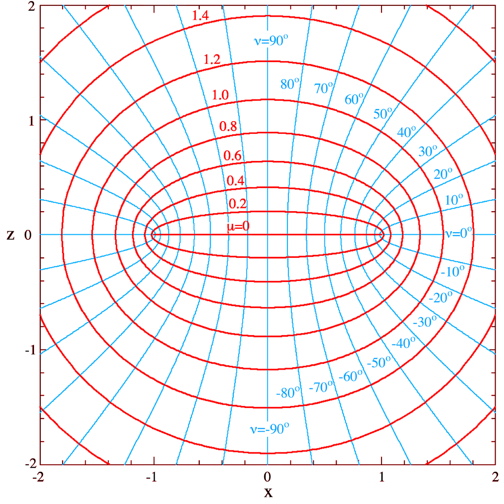
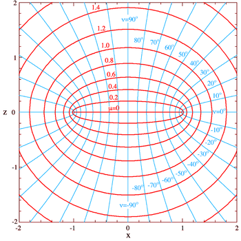Figure 2: Plot of the oblate spheroidal coordinates μ and ν in the x-z plane, where φ is zero and a equals one. The curves of constant μ form red ellipses, whereas those of constant ν form cyan half-hyperbolae in this plane. The z-axis runs vertically and separates the foci; the coordinates z and ν always have the same sign. The surfaces of constant μ and ν in three dimensions are obtained by rotation about the z-axis, and are the red and blue surfaces, respectively, in Figure 1.

The most common definition of oblate spheroidal coordinates (μ, ν, φ) is

$x = a \ \cosh \mu \ \cos \nu \ \cos \phi$

$y = a \ \cosh \mu \ \cos \nu \ \sin \phi$

$z = a \ \sinh \mu \ \sin \nu$

where μ is a nonnegative real number and the angle ν lies between ±90°. The azimuthal angle φ can fall anywhere on a full circle, between ±180°. These coordinates are favored over the alternatives below because they are not degenerate; every point in Cartesian coordinates (x, y, z) is described by exactly one set of coordinates (μ, ν, φ), and vice versa.

Coordinate surfaces

The surfaces of constant μ form oblate spheroids, by the trigonometric identity

$\frac{x^{2} + y^{2}}{a^{2} \cosh^{2} \mu} + \frac{z^{2}}{a^{2} \sinh^{2} \mu} = \cos^{2} \nu + \sin^{2} \nu = 1$

since they are ellipses rotated about the z-axis, which separates their foci. An ellipse in the x-z plane (Figure 2) has a major semiaxis of length a cosh μ along the x-axis, whereas its minor semiaxis has length a sinh μ along the z-axis. The foci of all the ellipses in the x-z plane are located on the x-axis at ±a.

Similarly, the surfaces of constant ν form one-sheet half hyperboloids of revolution by the hyperbolic trigonometric identity

$\frac{x^{2} + y^{2}}{a^{2} \cos^{2} \nu} - \frac{z^{2}}{a^{2} \sin^{2} \nu} = \cosh^{2} \mu - \sinh^{2} \mu = 1$

For positive ν, the half-hyperboloid is above the x-y plane (i.e., has positive z) whereas for negative ν, the half-hyperboloid is below the x-y plane (i.e., has negative z). Geometrically, the angle ν corresponds to the angle of the asymptotes of the hyperbola. The foci of all the hyperbolae are likewise located on the x-axis at ±a.

Inverse transformation

The (μ, ν, φ) coordinates may be calculated from the Cartesian coordinates (x, y, z) as follows. The azimuthal angle φ is given by the formula

$\tan \phi = \frac{y}{x}$

The cylindrical radius ρ of the point P is given by

ρ² = x² + y²

and its distances to the foci in the plane defined by φ is given by

$d_{1}^{2} = (\rho + a)^{2} + z^{2}$

$d_{2}^{2} = (\rho - a)^{2} + z^{2}$

The remaining coordinates μ and ν can be calculated from the equations

$\cosh \mu = \frac{d_{1} + d_{2}}{2a}$

$\cos \nu = \frac{d_{1} - d_{2}}{2a}$

where the sign of μ is always non-negative, and the sign of ν is the same as that of z.

Scale factors

The scale factors for the coordinates μ and ν are equal

$h_{\mu} = h_{\nu} = a\sqrt{\sinh^{2}\mu + \sin^{2}\nu}$

whereas the azimuthal scale factor equals

$h_{\phi} = a \cosh\mu \ \cos\nu$

Consequently, an infinitesimal volume element equals

$dV = a^{3} \cosh\mu \ \cos\nu \ \left( \sinh^{2}\mu + \sin^{2}\nu \right) d\mu d\nu d\phi$

and the Laplacian can be written

$\nabla^{2} \Phi = \frac{1}{a^{2} \left( \sinh^{2}\mu + \sin^{2}\nu \right)} \left[ \frac{1}{\cosh \mu} \frac{\partial}{\partial \mu} \left( \cosh \mu \frac{\partial \Phi}{\partial \mu} \right) + \frac{1}{\cos \nu} \frac{\partial}{\partial \nu} \left( \cos \nu \frac{\partial \Phi}{\partial \nu} \right) \right] + \frac{1}{a^{2} \left( \cosh^{2}\mu\cos^{2}\nu \right)} \frac{\partial^{2} \Phi}{\partial \phi^{2}}$

Other differential operators such as $\nabla \cdot \mathbf{F}$ and $\nabla \times \mathbf{F}$ can be expressed in the coordinates (μ, ν, φ) by substituting the scale factors into the general formulae found in orthogonal coordinates.

Definition (ζ, ξ, φ)

Another set of oblate spheroidal coordinates (ζ,ξ,ϕ) are sometimes used where ζ = sinh μ and ξ = sin ν (Smythe 1968). The curves of constant ζ are oblate spheroids and the curves of constant ξ are the hyperboloids of revolution. The coordinate ζ is restricted by $0 \le \zeta < \infty$ and ξ is restricted by $-1 \le \xi < 1$.

The relationship to Cartesian coordinates is

$x = a\sqrt{(1+\zeta^2)(1-\xi^2)}\,\cos \phi\,$

$y = a\sqrt{(1+\zeta^2)(1-\xi^2)}\,\sin \phi\,$

$z = a \zeta \xi\,$

Scale factors

The scale factors for (ζ,ξ,φ) are:

$h_{\zeta} = a\sqrt{\frac{\zeta^2 + \xi^2}{1+\zeta^2}}$

$h_{\xi} = a\sqrt{\frac{\zeta^2 + \xi^2}{1 - \xi^2}}$

$h_{\phi} = a\sqrt{(1+\zeta^2)(1 - \xi^2)}$

Knowing the scale factors, various functions of the coordinates can be calculated by the general method outlined in the orthogonal coordinates article. The infinitesimal volume element is:

$dV = a^{3} (\zeta^2+\xi^2)\,d\zeta\,d\xi\,d\phi$

The gradient is:

$\nabla V = \frac{1}{h_{\zeta}} \frac{\partial V}{\partial \zeta} \,\hat{\zeta}+ \frac{1} {h_{\xi}} \frac{\partial V}{\partial \xi} \,\hat{\xi}+ \frac{1} {h_{\phi}} \frac{\partial V}{\partial \phi} \,\hat{\phi}$

The divergence is:

$\nabla \mathbf{F} = \frac{1}{a(\zeta^2+\xi^2)} \left\{ \frac{\partial}{\partial \zeta} \left(\sqrt{1+\zeta^2}\sqrt{\zeta^2+\xi^2}F_\zeta\right) + \frac{\partial} {\partial \xi} \left(\sqrt{1-\xi^2}\sqrt{\zeta^2+\xi^2}F_\xi\right) \right\} +\frac{1}{\sqrt{1+\zeta^2}\sqrt{1-\xi^2}} \frac{\partial F_\phi}{\partial \phi}$

and the Laplacian equals

$\nabla^{2} V = \frac{1}{a^2 \left( \zeta^2 + \xi^2 \right)} \left\{ \frac{\partial}{\partial \zeta} \left[ \left(1+\zeta^2\right) \frac{\partial V}{\partial \zeta} \right] + \frac{\partial}{\partial \xi} \left[ \left( 1 - \xi^2 \right) \frac{\partial V}{\partial \xi} \right] \right\} + \frac{1}{a^2 \left( 1+\zeta^2 \right) \left( 1 - \xi^{2} \right)} \frac{\partial^2 V}{\partial \phi^{2}}$

Oblate spheroidal harmonics

As is the case with spherical coordinates and spherical harmonics, Laplace's equation may be solved by the method of separation of variables to yield solutions in the form of oblate spheroidal harmonics, which are convenient to use when boundary conditions are defined on a surface with a constant oblate spheroidal coordinate.

Following the technique of separation of variables, a solution to Laplace's equation is written:

$V=Z(\zeta)\,\Xi(\xi)\,\Phi(\phi)\,$

This yields three separate differential equations in each of the variables:

$\frac{d}{d\zeta}\left[(1+\zeta^2)\frac{dZ }{d\zeta}\right]+\frac{m^2Z }{1+\zeta^2}-n(n+1)Z =0$

$\frac{d}{d\xi }\left[(1-\xi^2 )\frac{d\Xi}{d\xi }\right]-\frac{m^2\Xi}{1-\xi^2 }+n(n+1)\Xi=0$

$\frac{d^2\Phi}{d\phi^2}=-m^2\Phi$

where m is a constant which is an integer because the φ variable is periodic with period 2π. n will then be an integer. The solution to these equations are:

$Z_{mn} =A_1P_n^m(i\zeta)+A_2Q_n^m(i\zeta)$

$\Xi_{mn} =A_3P_n^m(\xi)+A_4Q_n^m(\xi)$

$\Phi_m =A_5e^{im\phi}+A_6e^{-im\phi}\,$

where the A_i are constants and $P_n^m(z)$ and $Q_n^m(z)$ are associated Legendre polynomials of the first and second kind respectively. The product of the three solutions is called an oblate spheroidal harmonic and the general solution to Laplace's equation is written:

$V=\sum_{n=0}^\infty\sum_{m=0}^\infty\,Z_{mn}(\zeta)\,\Xi_{mn}(\xi)\,\Phi_m(\phi)$

The constants will combine to yield only four independent constants for each harmonic.

Definition (σ, τ, φ)

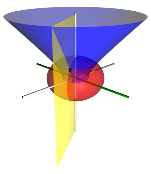
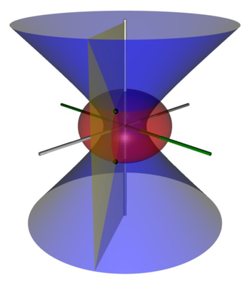Figure 3: Coordinate isosurfaces for a point P (shown as a black sphere) in the alternative oblate spheroidal coordinates (σ, τ, φ). As before, the oblate spheroid corresponding to σ is shown in red, and φ measures the azimuthal angle between the green and yellow half-planes. However, the surface of constant τ is a full one-sheet hyperboloid, shown in blue. This produces a two-fold degeneracy, shown by the two black spheres located at (x, y, ±z).

An alternative and geometrically intuitive set of oblate spheroidal coordinates (σ, τ, φ) are sometimes used, where σ = cosh μ and τ = cos ν.^[1] Therefore, the coordinate σ must be greater than or equal to one, whereas τ must lie between ±1, inclusive. The surfaces of constant σ are oblate spheroids, as were those of constant μ, whereas the curves of constant τ are full hyperboloids of revolution, including the half-hyperboloids corresponding to ±ν. Thus, these coordinates are degenerate; two points in Cartesian coordinates (x, y, ±z) map to one set of coordinates (σ, τ, φ). This two-fold degeneracy in the sign of z is evident from the equations transforming from oblate spheroidal coordinates to the Cartesian coordinates

$x = a\sigma\tau \cos \phi\,$

$y = a\sigma\tau \sin \phi\,$

$z^{2} = a^{2} \left( \sigma^{2} - 1 \right) \left(1 - \tau^{2} \right)$

The coordinates σ and τ have a simple relation to the distances to the focal ring. For any point, the sum d₁ + d₂ of its distances to the focal ring equals 2aσ, whereas their difference d₁ − d₂ equals 2aτ. Thus, the "far" distance to the focal ring is a(σ + τ), whereas the "near" distance is a(σ − τ).

Coordinate surfaces

Similar to its counterpart μ, the surfaces of constant σ form oblate spheroids

$\frac{x^{2} + y^{2}}{a^{2} \sigma^{2}} + \frac{z^{2}}{a^{2} \left(\sigma^{2} -1\right)} = 1$

Similarly, the surfaces of constant τ form full one-sheet hyperboloids of revolution

$\frac{x^{2} + y^{2}}{a^{2} \tau^{2}} - \frac{z^{2}}{a^{2} \left( 1 - \tau^{2} \right)} = 1$

Scale factors

The scale factors for the alternative oblate spheroidal coordinates (σ,τ,ϕ) are

$h_{\sigma} = a\sqrt{\frac{\sigma^{2} - \tau^{2}}{\sigma^{2} - 1}}$

$h_{\tau} = a\sqrt{\frac{\sigma^{2} - \tau^{2}}{1 - \tau^{2}}}$

whereas the azimuthal scale factor is h_ϕ = aστ.

Hence, the infinitesimal volume element can be written

$dV = a^{3} \sigma \tau \frac{\sigma^{2} - \tau^{2}}{\sqrt{\left( \sigma^{2} - 1 \right) \left( 1 - \tau^{2} \right)}} d\sigma d\tau d\phi$

and the Laplacian equals

$\nabla^{2} \Phi = \frac{1}{a^{2} \left( \sigma^{2} - \tau^{2} \right)} \left\{ \frac{\sqrt{\sigma^{2} -1}}{\sigma} \frac{\partial}{\partial \sigma} \left[ \left( \sigma\sqrt{\sigma^{2} - 1} \right) \frac{\partial \Phi}{\partial \sigma} \right] + \frac{\sqrt{1 - \tau^{2}}}{\tau} \frac{\partial}{\partial \tau} \left[ \left( \tau\sqrt{1 - \tau^{2}} \right) \frac{\partial \Phi}{\partial \tau} \right] \right\} + \frac{1}{a^{2} \sigma^{2} \tau^{2} } \frac{\partial^{2} \Phi}{\partial \phi^{2}}$

Other differential operators such as $\nabla \cdot \mathbf{F}$ and $\nabla \times \mathbf{F}$ can be expressed in the coordinates (σ,τ) by substituting the scale factors into the general formulae found in orthogonal coordinates.

As is the case with spherical coordinates, Laplaces equation may be solved by the method of separation of variables to yield solutions in the form of oblate spheroidal harmonics, which are convenient to use when boundary conditions are defined on a surface with a constant oblate spheroidal coordinate (See Smythe, 1968).

References

1. ^ Abramowitz and Stegun, p. 752.

Bibliography

No angles convention

• Morse PM, Feshbach H (1953). Methods of Theoretical Physics, Part I. New York: McGraw-Hill. p. 662.  Uses ξ₁ = a sinh μ, ξ₂ = sin ν, and ξ₃ = cos φ.
• Zwillinger D (1992). Handbook of Integration. Boston, MA: Jones and Bartlett. p. 115. ISBN 0-86720-293-9.  Same as Morse & Feshbach (1953), substituting u_k for ξ_k.
• Smythe, WR (1968). Static and Dynamic Electricity (3rd ed. ed.). New York: McGraw-Hill. 
• Sauer R, Szabó I (1967). Mathematische Hilfsmittel des Ingenieurs. New York: Springer Verlag. p. 98. LCCN 67-25285.  Uses hybrid coordinates ξ = sinh μ, η = sin ν, and φ.

Angle convention

• Korn GA, Korn TM (1961). Mathematical Handbook for Scientists and Engineers. New York: McGraw-Hill. p. 177. LCCN 59-14456.  Korn and Korn use the (μ, ν, φ) coordinates, but also introduce the degenerate (σ, τ, φ) coordinates.
• Margenau H, Murphy GM (1956). The Mathematics of Physics and Chemistry. New York: D. van Nostrand. p. 182. LCCN 55-10911.  Like Korn and Korn (1961), but uses colatitude θ = 90° - ν instead of latitude ν.
• Moon PH, Spencer DE (1988). "Oblate spheroidal coordinates (η, θ, ψ)". Field Theory Handbook, Including Coordinate Systems, Differential Equations, and Their Solutions (corrected 2nd ed., 3rd print ed. ed.). New York: Springer Verlag. pp. 31–34 (Table 1.07). ISBN 0-387-02732-7.  Moon and Spencer use the colatitude convention θ = 90° - ν, and re-name φ as ψ.

Unusual convention

• Landau LD, Lifshitz EM, Pitaevskii LP (1984). Electrodynamics of Continuous Media (Volume 8 of the Course of Theoretical Physics) (2nd edition ed.). New York: Pergamon Press. pp. 19–29. ISBN 978-0750626347.  Treats the oblate spheroidal coordinates as a limiting case of the general ellipsoidal coordinates. Uses (ξ, η, ζ) coordinates that have the units of distance squared.

External links

• MathWorld description of oblate spheroidal coordinates