- Space-filling curve
-
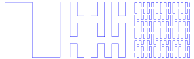 3 iterations of a Peano curve construction, whose limit is a space-filling curve.
In mathematical analysis, a space-filling curve is a curve whose range contains the entire 2-dimensional unit square (or more generally an N-dimensional hypercube). Because Giuseppe Peano (1858–1932) was the first to discover one, space-filling curves in the 2-dimensional plane are commonly called Peano curves.
Contents
Definition
Intuitively, a continuous curve in 2 or 3 (or higher) dimensions can be thought of as the path of a continuously moving point. To eliminate the inherent vagueness of this notion Jordan in 1887 introduced the following rigorous definition, which has since been adopted as the precise description of the notion of a continuous curve:
- A curve (with endpoints) is a continuous function whose domain is the unit interval [0, 1].
In the most general form, the range of such a function may lie in an arbitrary topological space, but in the most common cases, the range will lie in a Euclidean space such as the 2-dimensional plane (a planar curve) or the 3-dimensional space (space curve).
Sometimes, the curve is identified with the range or image of the function (the set of all possible values of the function), instead of the function itself. It is also possible to define curves without endpoints to be a continuous function on the real line (or on the open unit interval (0, 1)).
History
In 1890, Peano discovered a densely self-intersecting curve that passes through every point of the unit square. His purpose was to construct a continuous mapping from the unit interval onto the unit square. Peano was motivated by Georg Cantor's earlier counterintuitive result that the infinite number of points in a unit interval is the same cardinality as the infinite number of points in any finite-dimensional manifold, such as the unit square. The problem Peano solved was whether such a mapping could be continuous; i.e., a curve that fills a space.
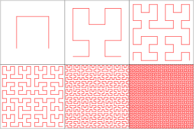 Six iterations of the Hilbert curve construction, whose limiting space-filling curve was devised by mathematician David Hilbert.
It was common to associate the vague notions of thinness and 1-dimensionality to curves; all normally encountered curves were piecewise differentiable (that is, have piecewise continuous derivatives), and such curves cannot fill up the entire unit square. Therefore, Peano's space-filling curve was found to be highly counterintuitive.
From Peano's example, it was easy to deduce continuous curves whose ranges contained the n-dimensional hypercube (for any positive integer n). It was also easy to extend Peano's example to continuous curves without endpoints which filled the entire n-dimensional Euclidean space (where n is 2, 3, or any other positive integer).
Most well-known space-filling curves are constructed iteratively as the limit of a sequence of piecewise linear continuous curves, each one more closely approximating the space-filling limit.
Peano's ground-breaking paper contained no illustrations of his construction, which is defined in terms of ternary expansions and a mirroring operator. But the graphical construction was perfectly clear to him—he made an ornamental tiling showing a picture of the curve in his home in Turin. Peano's paper also ends by mentioning (without proof) that the technique can be extended to other odd bases besides base 3. His choice to avoid any appeal to graphical visualization was no doubt motivated by a desire for a well-founded, completely rigorous proof owing nothing to pictures. At that time (the beginning of the foundation of general topology), graphical arguments were still included in proofs, yet were becoming a hindrance to understanding often counter-intuitive results.
A year later, David Hilbert published in the same journal a variation of Peano's construction. Hilbert's paper was the first to include a picture helping to visualize the construction technique, essentially the same as illustrated here. The analytic form of the Hilbert curve, however, is more complicated than Peano's.
Outline of the construction of a space-filling curve
Let
 denote the Cantor space
  .
.We start with a continuous function
 from the Cantor space onto the entire unit interval
 ![\scriptstyle [0,\, 1]](b/9bb589b580372e9075bc87f420e118b0.png) . (The restriction of the Cantor function to the Cantor set is an example of such a function.) From it, we get a continuous function
. (The restriction of the Cantor function to the Cantor set is an example of such a function.) From it, we get a continuous function  from the topological product
  onto the entire unit square
 ![\scriptstyle [0,\, 1] \;\times\; [0,\, 1]](9/7897f570910548b39cb4c22d4f8f6486.png) by setting
by setting- H(x,y) = (h(x),h(y)).
Since the Cantor set is homeomorphic to the product
 , there is a continuous bijection
  from the Cantor set onto . The composition
  of and is a continuous function mapping the Cantor set onto the entire unit square. (Alternatively, we could use the theorem that every compact metric space is a continuous image of the Cantor set to get the function .)
Finally, one can extend
to a continuous function  whose domain is the entire unit interval . This can be done either by using the Tietze extension theorem on each of the components of , or by simply extending "linearly" (that is, on each of the deleted open interval
  in the construction of the Cantor set, we define the extension part of on to be the line segment within the unit square joining the values
  and
and  ).
).Properties
A space-filling curve must be everywhere self-intersecting in the technical sense that the curve is not injective. If a curve is not injective, then one can find two subcurves of the curve, each obtained by considering the images of two disjoint segments from the curve's domain (the unit line segment). The two subcurves intersect if the intersection of the two images is non-empty. One might be tempted to think that the meaning of curves intersecting is that they necessarily cross each other, like the intersection point of two non-parallel lines, from one side to the other. However, two curves (or two subcurves of one curve) may contact one another without crossing, as, for example, a line tangent to a circle does.
A non-self-intersecting continuous curve cannot fill the unit square because that will make the curve a homeomorphism from the unit interval onto the unit square (any continuous bijection from a compact space onto a Hausdorff space is a homeomorphism). But a unit-square has no cut-point, and so cannot be homeomorphic to the unit interval, in which all points except the endpoints are cut-points.
For the classic Peano and Hilbert space-filling curves, where two subcurves intersect (in the technical sense), there is self-contact without self-crossing. A space-filling curve can be (everywhere) self-crossing if its approximation curves are self-crossing. A space-filling curve's approximations can be self-avoiding, as the figures above illustrate. In 3 dimensions, self-avoiding approximation curves can even contain knots. Approximation curves remain within a bounded portion of n-dimensional space, but their lengths increase without bound.
Space-filling curves are special cases of fractal constructions. No differentiable space-filling curve can exist. Roughly speaking, differentiability puts a bound on how fast the curve can turn.
Proof that a square and its side contain the same number of points
The highly counterintuitive result that the cardinality of a unit interval is the same as the cardinality of any finite-dimensional manifold, such as the unit square, was first obtained by Cantor in 1878, but it can be more intuitively proved using space-filling curves.
Intuitively, consider that the main difficulty resided in showing that a function of the unit interval can fill a square, a cube, or a hypercube, and this task was successfully accomplished by Peano. Indeed, being self-intersecting, his curves even manage to "overfill" the square. In other words, although Peano curves are not injective (because they overfill the space), they are surjective (because they fill it). This is true whether their self-intersection is self-crossing, or merely self-contacting.
Formally, a bijection between a set A and a set B is needed to prove that A and B have the same cardinality. Since space-filling curves "overfill" the space, they are not bijections. Thus, their existence is not a direct proof that a square (or cube or hypercube) contains as many points as its side. However, the right inverse of a space-filling curve is an injection, and can be used to obtain such a proof via the Cantor–Bernstein–Schroeder theorem, which asserts the existence of a bijection between A and B given that injections exist both from A into B and from B into A.
For instance, consider a space-filling curve that maps a unit interval A = [0, 1] onto a unit square B = [0, 1] × [0, 1]. This is a surjection from A into B, but one can define a right inverse for it which will be an injection from B into A. And x goes to (x,0) is an injection from A into B. Using the Cantor–Bernstein–Schroeder theorem, we get a bijection between A and B, the existence of which implies that A and B have the same cardinality.
One advantage of this proof is that, because an explicit definition of the right inverse is easily given, it does not require the use of the axiom of choice. For example, in the Hilbert curve each point in the square is the image of from one to four points in the line segment. When one of the coordinates is a rational number with a power of two in the denominator, that coordinate can be approached either from below or above giving two (not necessarily distinct) values for the preimage. Similarly, when both are such, then there are four (not necessarily distinct). Since the number of possible preimages for each point is finite (indeed less than or equal to four), one can just choose the smallest of them systematically, making the axiom of choice unnecessary.
Similarly, finite-dimensional space-filling curves can be used to prove, in general, that any finite-dimensional space contains the same number of points as any line or line segment.
The Hahn–Mazurkiewicz theorem
The Hahn–Mazurkiewicz theorem is the following characterization of spaces that are the continuous image of curves:
- A non-empty Hausdorff topological space is a continuous image of the unit interval if and only if it is a compact, connected, locally connected second-countable space.
Spaces that are the continuous image of a unit interval are sometimes called Peano spaces.
In many formulations of the Hahn–Mazurkiewicz theorem, second-countable is replaced by metrizable. These two formulations are equivalent. In one direction a compact Hausdorff space is a normal space and, by the Urysohn metrization theorem, second-countable then implies metrizable. Conversely a compact metric space is second-countable.
Kleinian groups
There are many natural examples of space-filling, or rather sphere-filling, curves in the theory of doubly degenerate Kleinian groups. For example, Cannon & Thurston (2007) showed that the circle at infinity of the universal cover of a fiber of a mapping torus of a pseudo-Anosov map is a sphere-filling curve. (Here the sphere is the sphere at infinity of hyperbolic 3-space.)
See also
- Dragon curve
- Gosper curve
- Moore curve
- Sierpiński curve
- Space-filling tree
- Hilbert R-tree
- Hilbert curve
- Bx-tree
- Z-order (Morton-order)
- List of fractals by Hausdorff dimension
- Osgood curve
References
- Cannon, James W.; Thurston, William P. (2007) [1982], "Group invariant Peano curves", Geometry & Topology 11: 1315–1355, doi:10.2140/gt.2007.11.1315, ISSN 1465-3060, MR2326947
- Hilbert, D. (1891), "Ueber die stetige Abbildung einer Line auf ein Flächenstück", Mathematische Annalen 38: 459–460, doi:10.1007/BF01199431.
- Mandelbrot, B. B. (1982), "Ch. 7: Harnessing the Peano Monster Curves", The Fractal Geometry of Nature, W. H. Freeman.
- McKenna, Douglas M. (1994), "SquaRecurves, E-Tours, Eddies, and Frenzies: Basic Families of Peano Curves on the Square Grid", in Guy, Richard K.; Woodrow, Robert E., The Lighter Side of Mathematics: Proceedings of the Eugene Strens Memorial Conference on Recreational Mathematics and its History, Mathematical Association of America, pp. 49–73, ISBN 9780883855164.
- Peano, G. (1890), "Sur une courbe, qui remplit toute une aire plane", Mathematische Annalen 36 (1): 157–160, doi:10.1007/BF01199438.
- Sagan, Hans (1994), Space-Filling Curves, Springer-Verlag, ISBN 0387942653, MR1299533.
External links
Java applets:
- Peano Plane Filling Curves at cut-the-knot
- Hilbert's and Moore's Plane Filling Curves at cut-the-knot
- All Peano Plane Filling Curves at cut-the-knot
Categories:- Continuous mappings
- Fractal curves


Wikimedia Foundation. 2010.