Monochromatic electromagnetic plane wave

In general relativity, the monochromatic electromagnetic plane wave spacetime is the analog of the monochromatic plane waves known from Maxwell's theory. The precise definition of the solution is a bit complicated, but very instructive.

Any exact solution of the Einstein field equation which models an electromagnetic field must take into account all gravitational effects of the energy of the electromagnetic field itself. If there is no matter and no non-gravitational fields present other than the electromagnetic field, this means that we must simultaneously solve the Einstein field equation and the (curved spacetime, source-free) Maxwell field equations.

In Maxwell's theory of electromagnetism, one of the most important types of an electromagnetic field are those representing electromagnetic radiation. Of these, the most important examples are the electromagnetic plane waves, in which the radiation has planar wavefronts moving in a specific direction at the speed of light. Of these, the most basic are the monochromatic plane waves, in which only one frequency component is present. This is precisely the phenomenon which our solution will model in terms of general relativity.

Definition of the solution

The metric tensor of the unique exact solution modeling a linearly polarized electromagnetic plane wave with amplitude q and frequency ω can be written, in terms of Rosen coordinates, in the form

$ds^2 = -2 \, du \, dv + C\left(\frac{q^2}{\omega^2}, \frac{2q^2}{\omega^2}, \omega u \right)^2 \, \left( dx^2 + dy^2 \right)$

$-\infty < v,x,y < \infty, -u_0 < u < u_0$

where $\xi=\frac{u_0}{\omega}$ is the first positive root of C(a,2a,ξ) = 0 where $a=\frac{q^2}{\omega^2}$. In this chart, $\partial_u, \partial_v$ are null coordinate vectors while $\partial_x, \partial_y$ are spacelike coordinate vectors.

Here, the Mathieu cosine C(a,b,ξ) is an even function which solves the Mathieu equation and also takes the value C(a,b,0) = 1. Despite the name, this function is not periodic, and it cannot be written in terms of sinusoidal or even hypergeometric functions. (See Mathieu function for more about the Mathieu cosine function.)

In our expression for the metric, note that $\partial_u, \, \partial_v$ are null vector fields. Therefore $\partial_u+\partial_v$ is a timelike vector field, while $\partial_u-\partial_v, \; \partial_x, \; \partial_y$ are spacelike vector fields.

To define the electromagnetic field, we may take the electromagnetic four-vector potential

$\vec{A} = \frac{ \sqrt{2} a \int C\left( \frac{u^2}{\omega^2}, \frac{q^2}{2\omega^2}, \omega u \right) \, \sin(\omega u) \, du }{ C\left( \frac{q^2}{\omega^2}, \frac{q^2}{2\omega^2}, \omega u \right)} \; \partial_x$

We now have the complete specification of a mathematical model formulated in general relativity.

Local isometries

Our spacetime is modeled by a Lorentzian manifold which has some remarkable symmetries. Namely, our spacetime admits a six dimensional Lie group of self-isometries. This group is generated by a six dimensional Lie algebra of Killing vector fields. A convenient basis consists of one null vector field,

$\vec{\xi}_1 = \partial_v$

three spacelike vector fields,

$\vec{\xi}_2 = \partial_x, \; \vec{\xi}_3 = \partial_y, \; \vec{\xi}_4 = -y \, \partial_x + x \, \partial_y$

and two additional vector fields,

$\vec{\xi}_5 = x \, \partial_v + \int \frac {du} { C \left( \frac{q^2}{\omega^2}, \frac{q^2}{2\omega^2}, \omega u \right) } \, \partial_x$

$\vec{\xi}_6 = y \, \partial_v + \int \frac {du} { C \left( \frac{q^2}{\omega^2}, \frac{q^2}{2\omega^2}, \omega u \right) } \, \partial_y$

Here, $\vec{\xi}_2, \, \vec{\xi}_3, \, \vec{\xi}_4$ generate the Euclidean group, acting within each planar wavefront, which justifies the name plane wave for this solution. Also $\vec{\xi}_5, \, \vec{\xi}_6$ show that all nontranverse directions are equivalent. This corresponds to the well-known fact that in flat spacetime, two colliding plane waves always collide head-on when represented in the appropriate Lorentz frame.

For future reference we note that this six dimensional group of self-isometries acts transitively, so that our spacetime is homogeneous. However, it is not isotropic, since the transverse directions are distinguished from the non-transverse ones.

A family of inertial observers

The frame field

$\vec{e}_0 = \frac{1}{\sqrt{2}} \left( \partial_u + \partial_v \right)$

$\vec{e}_1 = \frac{1}{\sqrt{2}} \left( -\partial_u + \partial_v \right)$

$\vec{e}_2 = \frac{1}{C\left(\frac{q^2}{\omega^2}, \, \frac{2q^2}{\omega^2}, \, \omega u \right)} \partial_x$

$\vec{e}_3 = \frac{1}{C\left(\frac{q^2}{\omega^2}, \, \frac{2q^2}{\omega^2}, \, \omega u \right)} \partial_y$

represents the local Lorentz frame defined by a family of nonspinning inertial observers. That is,

$\nabla_{\vec{e}_0} \vec{e}_0 = 0$

which means that the integral curves of the timelike unit vector field e₀ are timelike geodesics, and also

$\nabla_{\vec{e}_0} \vec{e}_1 = \nabla_{\vec{e}_0} \vec{e}_2 = \nabla_{\vec{e}_0} \vec{e}_3 = 0$

which means that the spacelike unit vector fields e₁,e₂,e₃ are nonspinning. (They are Fermi-Walker transported.) Here, $\vec{e}_0$ is a timelike unit vector field, while $\vec{e}_1, \, \vec{e}_2, \, \vec{e}_3$ are spacelike unit vector fields.

Nonspinning inertial frames are as close as we can come in curved spacetimes to the usual Lorentz frames known from special relativity, where Lorentz transformations are simply changes from one Lorentz frame to another.

The electromagnetic field

With respect to our frame, the electromagnetic field obtained from the potential given above is

$\vec{E} = q \, \sin(\omega u) \, \vec{e}_2$

$\vec{B} = -q \, \sin(\omega u) \, \vec{e}_3$

This electromagnetic field is a source-free solution of the Maxwell field equations on the particular curved spacetime which is defined by the metric tensor above. It is a null solution, and it represents a transverse sinusoidal electromagnetic plane wave with amplitude q and frequency ω, traveling in the e₁ direction. When we

• compute the stress-energy tensor T^ab for the given electromagnetic field,
• compute the Einstein tensor G^ab for the given metric tensor,

we find that the Einstein field equation $G^{ab} = 8 \pi \, T^{ab}$ is satisfied. This is what we mean by saying that we have an exact electrovacuum solution.

In terms of our frame, the stress-energy tensor turns out to be

$T^{\hat{j} \hat{k}} = \frac{q^2 \sin(\omega u)^2}{4 \pi} \, \left[ \begin{matrix} 1&1&0&0\\1&1&0&0\\0&0&0&0\\0&0&0&0 \end{matrix} \right]$

Notice that this is exactly the same expression that we would find in classical electromagnetism (where we neglect the gravitational effects of the electromagnetic field energy) for the null field given above; the only difference is that now our frame is a anholonomic (orthonormal) basis on a curved spacetime, rather than a coordinate basis in flat spacetime. (See frame fields.)

Relative motion of the observers

The Rosen chart is said to be comoving with our family of inertial nonspinning observers, because the coordinates $v-u,\, x, \, y$ are all constant along each world line, given by an integral curve of the timelike unit vector field $\vec{X} = \vec{e}_0$. Thus, in the Rosen chart, these observers might appear to be motionless. But in fact they are in relative motion with respect to one another. To see this, we should compute their expansion tensor with respect to the frame given above. This turns out to be

$\theta[\vec{X}]_{\hat{i} \hat{j}} = \frac{\omega}{\sqrt{2}} \, \frac{C^\prime( \frac{q^2}{\omega^2}, \frac{q^2}{2 \omega^2}, \omega u)}{C( \frac{q^2}{\omega^2}, \frac{q^2}{2 \omega^2}, \omega u)} \, \operatorname{diag} (0,1,1)$

where $C^\prime(a,q,\xi) = \frac{\partial C(a,q,\xi)}{\partial \xi}$. The nonvanishing components are identical, and are

1. concave down on − u₀ < u < u₀
2. vanish at u = 0.

Physically, this means that a small spherical 'cloud' of our inertial observers hovers momentarily at u = 0 and then begin to collapse, eventually passing through one another at u = u₀. If we imagine them as forming a three dimensional cloud of uniformly distributed test particles, this collapse occurs orthogonal to the direction of propagation of the wave. The cloud exhibits no relative motion in the direction of propagation, so this is a purely transverse motion.

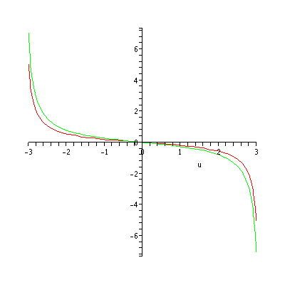
For $\frac{q}{\omega} \ll 1$ (the shortwave approximation), we have approximately

$g_{xx} \approx \cos(q u)^2$

$\theta[\vec{X}]_{22} \approx -q \, \tan(q u)$

For example, with q = 1 / 2,ω = 5, we have

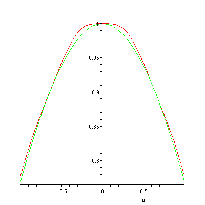
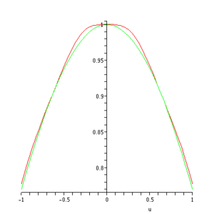Transverse metric tensor component.

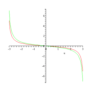Transverse expansion tensor component.

where the exact expressions plotted in red and the shortwave approximations in green.

The vorticity tensor of our congruence vanishes identically, so the world lines of our observers are hypersurface orthogonal. The three-dimensional Riemann tensor of the hyperslices is given, with respect to our frame, by

${{}^3 R}_{1212} = {{}^3 R}_{1313} = q^2 \, \sin(\omega u)^2$

${{}^3 R}_{2323} = \frac{-\omega^2}{2} \, \frac{C^\prime \left( \frac{q^2}{\omega^2}, \frac{q^2}{2\omega^2}, \omega u \right)^2}{C\left( \frac{q^2}{\omega^2}, \frac{q^2}{2\omega^2}, \omega u \right)^2}$

So the curvature splits neatly into wave (the sectional curvatures parallel to the direction of propagation) and background (the transverse sectional curvature).

The Riemann curvature tensor

In contrast, the Bel decomposition of the Riemann curvature tensor, taken with respect to $\vec{X} = \vec{e}_0$, is simplicity itself. The electrogravitic tensor, which directly represents the tidal accelerations, is

$E[\vec{X}]_{\hat{m} \hat{n}} = q^2 \, \sin(\omega u)^2 \, \operatorname{diag} (0,1,1)$

The magnetogravitic tensor, which directly represents the spin-spin force on a gyroscope carried by one of our observers, is

$B[\vec{X}]_{\hat{m} \hat{n}} = q^2 \, \sin(\omega u)^2 \, \left[ \begin{matrix} 0&0&0\\0&0&-1\\0&1&0 \end{matrix} \right]$

(The topogravitic tensor, which represents the spatial sectional curvatures, agrees with the electrogravitic tensor.)

Looking back at our graph of the metric tensor, we can see that the tidal tensor produces small sinusoidal relative accelerations with period ω, which are purely transverse to the direction of propagation of the wave. The net gravitational effect over many periods is to produce an expansion and recollapse cycle of our family of inertial nonspining observers. This can be considered the effect of the background curvature produced by the wave.

This expansion and recollapse cycle is reminiscent of the expanding and recollapsing FRW cosmological models, and it occurs for a similar reason: the presence of nongravitational mass-energy. In the FRW models, this mass-energy is due to the mass of the dust particles; here, it is due to the field energy of the electromagnetic field. There, the expansion-recollapse cycle begins and ends with a strong scalar curvature singularity; here, we have a mere coordinate singularity (a circumstance which much confused Einstein and Rosen in 1937). In addition, here we have a small sinusoidal modulation of the expansion and recollapse.

Optical effects

A general principle concerning plane waves states you cannot see the wave train enter the station, but you can see it leave. That is, if you look through oncoming wavefronts at distant objects, you will see no optical distortion, but if you turn and look through departing wavefronts at distanct object, you will see optical distortions. Specifically, the null geodesic congruence generated by the null vector field $\vec{k} = \vec{e}_0 + \vec{e}_1$ has vanishing optical scalars, but the null geodesic congruence generated by $\vec{\ell} = \vec{e}_0 - \vec{e}_1$ has vanishing twist and shear scalars but nonvanishing expansion scalar

$\theta = \sqrt{2} \omega \, \frac{C^\prime \left( \frac{q^2}{\omega^2},\frac{q^2}{2 \omega^2},\omega u \right)}{C \left( \frac{q^2}{\omega^2}, \frac{q^2}{2 \omega^2}, \omega u \right)}$

This shows that when looking through departing wavefronts at distant objects, our inertial nonspinning observers will see their apparent size change exactly the same way as the expansion of the timelike geodesic congruence itself.

The Brinkmann chart

One way to quickly see the plausibility of the assertion that u = u₀ is a mere coordinate singularity is to recall that our spacetime is homogeneous, so that all events are equivalent. To confirm this directly, and to study from a different perspective the relative motion of our inertial nonspinning observers, we can apply the coordinate transformation

$u \rightarrow u$

$v \rightarrow v - \frac{\dot{r}}{2r} (x^2+y^2)$

$x \rightarrow x/r$

$y \rightarrow y/r$

where

$-\frac{\ddot{r}(u)}{r(u)} = q \sin(\omega u)^2$

This brings the solution into its representation in terms of Brinkmann coordinates:

$ds^2 = -q \, \sin(\omega u)^2 \, du^2 - 2 \, du \, dv + dx^2 + dy^2,$

$-\infty < u,v,x,y < \infty$

Since it can be shown that the new coordinates are geodesically complete, the Brinkmann coordinates define a global coordinate chart. In this chart, we can see that an infinite sequence of identical expansion-recollapse cycles occur!

Caustics

In the Brinkmann chart, our frame field becomes rather complicated:

$\vec{e}_0 = \frac{1}{\sqrt{2}} \, \left( \partial_u + \partial_v \right) + \frac{x^2+y^2}{\sqrt{2}} \, \left( -q^2 \sin(\omega u)^2 + \frac{\omega^2}{2} \, \frac{C^\prime \left( \frac{q^2}{\omega^2}, \frac{q^2}{2 \omega^2}, \omega u \right)^2}{C \left( \frac{q^2}{\omega^2}, \frac{q^2}{2 \omega^2}, \omega u \right)^2} \right) \, \partial_v$

$\; \; \; + \frac{\omega}{2} \, \frac{C^\prime \left( \frac{q^2}{\omega^2}, \frac{q^2}{2 \omega^2}, \omega u \right)}{C \left( \frac{q^2}{\omega^2}, \frac{q^2}{2 \omega^2}, \omega u \right)} \, \left( x \, \partial_x + y \, \partial_y \right)$

and so forth. Naturally, if we compute the expansion tensor, electrogravitic tensor, and so forth, we obtain exactly the same answers as before, but expressed in the new coordinates.

The simplicity of the metric tensor compared to the complexity of the frame is striking. The point is that we can more easily visualize the caustics formed by the relative motion of our observers in the new chart. The integral curves of the timelike unit geodesic vector field $\vec{X}=\vec{e}_0$ give the world lines of our observers. In the Rosen chart, these appear as vertical coordinate lines, since that chart is comoving.

To understand how this situation appears in the Brinkmann chart, notice that when ω is large, our timelike geodesic unit vector field becomes approximately

$\vec{X} \approx \frac{1}{\sqrt{2}} \, \left( \partial_u + \partial_v \right) - q \tan(q u) \, \left( x \partial_x + y \partial_y \right)$

$\; \; + \frac{x^2+y^2}{\sqrt{2}} \, \left( -q^2 \sin(\omega u)^2 + q^2 \tan(q u)^2 \right) \partial_v$

Suppressing the last term, we have

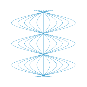Approximate motion of our family of observers, as represented in Brinkmann chart

$\vec{X} \approx \partial_t - q \tan(q u/\sqrt{2}) \, \left( x \partial_x + y \partial_y \right)$

We immediately obtain an integral curve which exhibits sinusoidal expansion and reconvergence cycles. See the figure, in which time is running vertically and we use the radial symmetry to suppress one spatial dimension. This figure shows why there is a coordinate singularity in the Rosen chart; the observers must actually pass by one another at regular intervals, which is obviously incompatible with the comoving property, so the chart breaks down at these places. Note that this figure incorrectly suggests that one observer is the 'center of attraction', as it were, but in fact they are all completely equivalent, due to the large symmetry group of this spacetime. Note too that the broadly sinusoidal relative motion of our observers is fully consistent with the behavior of the expansion tensor (with respect to the frame field corresponding to our family of observers) which was noted above.

It is worth noting that these somewhat tricky points confused no less a figure than Albert Einstein in his 1937 paper on gravitational waves (written long before the modern mathematical machinery used here was widely appreciated in physics).

Thus, in the Brinkmann chart, the world lines of our observers, in the shortwave case, are periodic curves which have the form of sinusoidals with period 2π / q, modulated by much smaller sinusoidal perturbations in the null direction $\partial_v$ and having a much shorter period, 2π / ω. The observers periodically expand and recollapse transversely to the direct of propagation; this motion is modulated by short period small amplitude perturbations.

Summary

Comparing our exact solution with the usual monochromatic electromagnetic plane wave as treated in special relativity (i.e., as a wave in flat spacetime, neglecting the gravitational effects of the energy of the electromagnetic field), we see that the striking new feature in general relativity is the expansion and collapse cycles experienced by our observers, which we can put down to background curvature, not any measurements made over short times and distances (on the order of the wavelength of the electromagnetic radiation).

See also

• Sticky bead argument, for an account of the 1937 paper by Einstein and Rosen alluded to above.

References

• Misner, Charles; Thorne, Kip S. & Wheeler, John Archibald (1973). Gravitation. San Francisco: W. H. Freeman. ISBN 0-7167-0344-0.  See section 35.11

Retrieved from "http://en.wikipedia.org/wiki/Monochromatic_electromagnetic_plane_wave"