Discrete wavelet transform

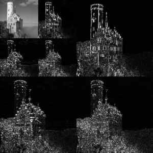An example of the 2D discrete wavelet transform that is used in JPEG2000. The original image is high-pass filtered, yielding the three large images, each describing local changes in brightness (details) in the original image. It is then low-pass filtered and downscaled, yielding an approximation image; this image is high-pass filtered to produce the three smaller detail images, and low-pass filtered to produce the final approximation image in the upper-left.

In numerical analysis and functional analysis, a discrete wavelet transform (DWT) is any wavelet transform for which the wavelets are discretely sampled. As with other wavelet transforms, a key advantage it has over Fourier transforms is temporal resolution: it captures both frequency and location information (location in time).

Examples

Haar wavelets

Main article: Haar wavelet

The first DWT was invented by the Hungarian mathematician Alfréd Haar. For an input represented by a list of 2ⁿ numbers, the Haar wavelet transform may be considered to simply pair up input values, storing the difference and passing the sum. This process is repeated recursively, pairing up the sums to provide the next scale: finally resulting in 2ⁿ − 1 differences and one final sum.

Daubechies wavelets

Main article: Daubechies wavelet

The most commonly used set of discrete wavelet transforms was formulated by the Belgian mathematician Ingrid Daubechies in 1988. This formulation is based on the use of recurrence relations to generate progressively finer discrete samplings of an implicit mother wavelet function; each resolution is twice that of the previous scale. In her seminal paper, Daubechies derives a family of wavelets, the first of which is the Haar wavelet. Interest in this field has exploded since then, and many variations of Daubechies' original wavelets were developed.

Others

Other forms of discrete wavelet transform include the non- or undecimated wavelet transform (where downsampling is omitted), the Newland transform (where an orthonormal basis of wavelets is formed from appropriately constructed top-hat filters in frequency space). Wavelet packet transforms are also related to the discrete wavelet transform. Complex wavelet transform is another form.

Properties

The Haar DWT illustrates the desirable properties of wavelets in general. First, it can be performed in O(n) operations; second, it captures not only a notion of the frequency content of the input, by examining it at different scales, but also temporal content, i.e. the times at which these frequencies occur. Combined, these two properties make the Fast wavelet transform (FWT) an alternative to the conventional Fast Fourier Transform (FFT).

Applications

The discrete wavelet transform has a huge number of applications in science, engineering, mathematics and computer science. Most notably, it is used for signal coding, to represent a discrete signal in a more redundant form, often as a preconditioning for data compression. Practical applications can also be found in signal processing of accelerations for gait analysis^[1].

Comparison with Fourier transform

See also: Discrete Fourier transform

To illustrate the differences and similarities between the discrete wavelet transform with the discrete Fourier transform, consider the DWT and DFT of the following sequence: (1,0,0,0), a unit impulse.

The DFT has orthogonal basis (DFT matrix):

 1  1  1  1
 1  0 –1  0
 0  1  0 –1
 1 –1  1 –1

while the DWT with Haar wavelets for length 4 data has orthogonal basis in the rows of:

 1  1  1  1
 1  1 –1 –1
 1 –1  0  0
 0  0  1 –1

(To simplify notation, whole numbers are used, so the bases are orthogonal but not orthonormal.)

Preliminary observations include:

• Wavelets have location – the (1,1,–1,–1) wavelet corresponds to “left side” versus “right side”, while the last two wavelets have support on the left side or the right side, and one is a translation of the other.
• Sinusoidal waves do not have location – they spread across the whole space – but do have phase – the second and third waves are translations of each other, corresponding to being 90° out of phase, like cosine and sine, of which these are discrete versions.

Decomposing the sequence with respect to these bases yields:

$\begin{align} (1,0,0,0) &= \frac{1}{4}(1,1,1,1)+\frac{1}{4}(1,1,-1,-1) + \frac{1}{2}(1,-1,0,0) \qquad\text{Haar DWT}\\ (1,0,0,0) &= \frac{1}{4}(1,1,1,1) + \frac{1}{2}(1,0,-1,0) + \frac{1}{4}(1,-1,1,-1) \qquad\text{DFT} \end{align}$

The DWT demonstrates the localization: the (1,1,1,1) term gives the average signal value, the (1,1,–1,–1) places the signal in the left side of the domain, and the (1,–1,0,0) places it at the left side of the left side, and truncating at any stage yields a downsampled version of the signal:

$\begin{align} &\left(\frac{1}{4},\frac{1}{4},\frac{1}{4},\frac{1}{4}\right)\\ &\left(\frac{1}{2},\frac{1}{2},0,0\right)\qquad\text{2-term truncation}\\ &\left(1,0,0,0\right) \end{align}$

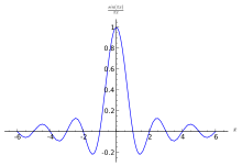The sinc function, showing the time domain artifacts (undershoot and ringing) of truncating a Fourier series.

The DFT, by contrast, expresses the sequence by the interference of waves of various frequencies – thus truncating the series yields a low-pass filtered version of the series:

$\begin{align} &\left(\frac{1}{4},\frac{1}{4},\frac{1}{4},\frac{1}{4}\right)\\ &\left(\frac{3}{4},\frac{1}{4},-\frac{1}{4},\frac{1}{4}\right)\qquad\text{2-term truncation}\\ &\left(1,0,0,0\right) \end{align}$

Notably, the middle approximation (2-term) differs. From the frequency domain perspective, this is a better approximation, but from the time domain perspective it has drawbacks – it exhibits undershoot – one of the values is negative, though the original series is non-negative everywhere – and ringing, where the right side is non-zero, unlike in the wavelet transform. On the other hand, the Fourier approximation correctly shows a peak, and all points are within 1 / 4 of their correct value, though all points have error. The wavelet approximation, by contrast, places a peak on the left half, but has no peak at the first point, and while it is exactly correct for half the values (reflecting location), it has an error of 1 / 2 for the other values.

This illustrates the kinds of trade-offs between these transforms, and how in some respects the DWT provides preferable behavior, particularly for the modeling of transients, which is of interest in applications.

Definition

One level of the transform

The DWT of a signal x is calculated by passing it through a series of filters. First the samples are passed through a low pass filter with impulse response g resulting in a convolution of the two:

$y[n] = (x * g)[n] = \sum\limits_{k = - \infty }^\infty {x[k] g[n - k]}.$

The signal is also decomposed simultaneously using a high-pass filter h. The outputs giving the detail coefficients (from the high-pass filter) and approximation coefficients (from the low-pass). It is important that the two filters are related to each other and they are known as a quadrature mirror filter.

However, since half the frequencies of the signal have now been removed, half the samples can be discarded according to Nyquist’s rule. The filter outputs are then subsampled by 2 (Mallat's and the common notation is the opposite, g- high pass and h- low pass):

$y_{\mathrm{low}} [n] = \sum\limits_{k = - \infty }^\infty {x[k] g[2 n - k]}$

$y_{\mathrm{high}} [n] = \sum\limits_{k = - \infty }^\infty {x[k] h[2 n - k]}$

This decomposition has halved the time resolution since only half of each filter output characterises the signal. However, each output has half the frequency band of the input so the frequency resolution has been doubled.

Block diagram of filter analysis

With the subsampling operator $\downarrow$

$(y \downarrow k)[n] = y[k n]$

the above summation can be written more concisely.

$y_{\mathrm{low}} = (x*g)\downarrow 2$

$y_{\mathrm{high}} = (x*h)\downarrow 2$

However computing a complete convolution x * g with subsequent downsampling would waste computation time.

The Lifting scheme is an optimization where these two computations are interleaved.

Cascading and Filter banks

This decomposition is repeated to further increase the frequency resolution and the approximation coefficients decomposed with high and low pass filters and then down-sampled. This is represented as a binary tree with nodes representing a sub-space with a different time-frequency localisation. The tree is known as a filter bank.

A 3 level filter bank

At each level in the above diagram the signal is decomposed into low and high frequencies. Due to the decomposition process the input signal must be a multiple of 2ⁿ where n is the number of levels.

For example a signal with 32 samples, frequency range 0 to f_n and 3 levels of decomposition, 4 output scales are produced:

Level	Frequencies	Samples
3	0 to fn / 8	4
	fn / 8 to fn / 4	4
2	fn / 4 to fn / 2	8
1	fn / 2 to fn	16

Frequency domain representation of the DWT

Other transforms

See also: Adam7 algorithm

The Adam7 algorithm, used for interlacing in the Portable Network Graphics (PNG) format, is a multiscale model of the data which is similar to a DWT with Haar wavelets.

Unlike the DWT, it has a specific scale – it starts from an 8×8 block, and it downsamples the image, rather than decimating (low-pass filtering, then downsampling). It thus offers worse frequency behavior, showing artifacts (pixelation) at the early stages, in return for simpler implementation.

Code examples

In its simplest form, the DWT is remarkably easy to compute.

The Haar wavelet in Java:

public static int[] discreteHaarWaveletTransform(int[] input) {
    // This function assumes that input.length=2^n, n>1
    int[] output = new int[input.length];
 
    for (int length = input.length >> 1; ; length >>= 1) {
        // length = input.length / 2^n, WITH n INCREASING to log(input.length) / log(2)
        for (int i = 0; i < length; ++i) {
            int sum = input[i * 2] + input[i * 2 + 1];
            int difference = input[i * 2] - input[i * 2 + 1];
            output[i] = sum;
            output[length + i] = difference;
        }
        if (length == 1) {
            return output;
        }
 
        //Swap arrays to do next iteration
        System.arraycopy(output, 0, input, 0, length << 1);
    }
}

Complete Java code for a 1-D and 2-D DWT using Haar, Daubechies, Coiflet, and Legendre wavelets is available from the open source project: JWave. Furthermore, a fast lifting implementation of the discrete biorthogonal CDF 9/7 wavelet transform in C, used in the JPEG 2000 image compression standard can be found here.

See also

• Wavelet series
• Wavelet compression
• List of wavelet-related transforms

Notes

References

• Stéphane Mallat, A Wavelet Tour of Signal Processing

1. ^ "Novel method for stride length estimation with body area network accelerometers", IEEE BioWireless 2011, pp. 79-82