DFT matrix

A DFT matrix is an expression of a discrete Fourier transform (DFT) as a matrix multiplication.

Definition

An N-point DFT is expressed as an N-by-N matrix multiplication as X = Wx, where x is the original input signal, and X is the DFT of the signal.

The transformation W of size $N\times N$ can be defined as $W = \left(\frac{\omega^{jk}}{\sqrt{N}}\right)_{j,k=0,\ldots,N-1}$, or equivalently:

$W = \frac{1}{\sqrt{N}} \begin{bmatrix} 1&1&1&1&\cdots &1 \\ 1&\omega&\omega^2&\omega^3&\cdots&\omega^{N-1} \\ 1&\omega^2&\omega^4&\omega^6&\cdots&\omega^{2(N-1)}\\ 1&\omega^3&\omega^6&\omega^9&\cdots&\omega^{3(N-1)}\\ \vdots&\vdots&\vdots&\vdots&&\vdots\\ 1&\omega^{N-1}&\omega^{2(N-1)}&\omega^{3(N-1)}&\cdots&\omega^{(N-1)(N-1)}\\ \end{bmatrix},$

where $\omega = e^{-\frac{2\pi i}{N}}$ is a primitive Nth root of unity in which $i=\sqrt{-1}$. This is the Vandermonde matrix for the roots of unity, up to the normalization factor. Note that the normalization factor in front of the sum ($1/\sqrt{N}$) and the sign of the exponent in ω are merely conventions, and differ in some treatments. All of the following discussion applies regardless of the convention, with at most minor adjustments. The only important thing is that the forward and inverse transforms have opposite-sign exponents, and that the product of their normalization factors be 1/N. However, the $1/\sqrt{N}$ choice here makes the resulting DFT matrix unitary, which is convenient in many circumstances.

Fast Fourier Transform algorithms utilize the symmetries of the matrix to reduce the time of multiplying a vector by this matrix, from the usual O(N²). Similar techniques can be applied for multiplications by matrices such as Hadamard matrix and the Walsh matrix.

Examples

Two-point

The two-point DFT is a simple case, in which the first entry is the DC (sum) and the second entry is the AC (difference).

$\frac{1}{\sqrt{2}} \begin{bmatrix} 1 & 1 \\ 1 & -1 \end{bmatrix}$

The first row performs the sum, and the second row performs the difference.

The factor of $1/\sqrt{2}$ is to make the transform unitary (see below).

Four-point

The four-point DFT matrix is as follows:

$\frac{1}{2} \begin{bmatrix} 1 & 1 & 1 & 1\\ 1 &-i &-1 & i\\ 1 & -1& 1 &-1\\ 1 & i &-1 & -i\end{bmatrix}.$

Eight-point

The first non-trivial integer power of two case is for 8 points:

$W= \frac{1}{\sqrt{8}} \begin{bmatrix} \omega^0 & \omega^0 &\omega^0 & \ldots & \omega^0 \\ \omega^0 & \omega^1 &\omega^2 & \ldots & \omega^7 \\ \omega^0 & \omega^2 &\omega^4 & \ldots & \omega^{14} \\ \omega^0 & \omega^3 &\omega^6 & \ldots & \omega^{21} \\ \omega^0 & \omega^4 &\omega^8 & \ldots & \omega^{28} \\ \omega^0 & \omega^5 &\omega^{10} & \ldots & \omega^{35} \\ \vdots & \vdots & \vdots & \ddots & \vdots \\ \omega^0 & \omega^7 &\omega^{14} & \ldots & \omega^{49} \\ \end{bmatrix}$

where

$\omega = e^{-\frac{2 \pi i}{8}} = \frac{1}{\sqrt{2}} - \frac{i}{\sqrt{2}}$

The following image depicts the DFT as a matrix multiplication, with elements of the matrix depicted by samples of complex exponentials:

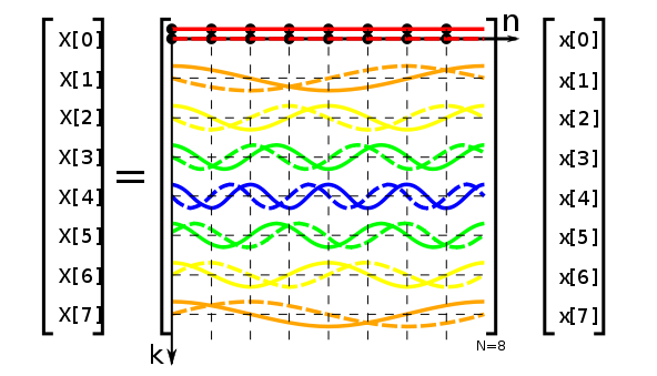
The real part (cosine wave) is denoted by a solid line, and the imaginary part (sine wave) by a dashed line.

The top row is all ones (scaled by $1/\sqrt{8}$ for unitarity), so it "measures" the DC component in the input signal. The next row is eight samples of negative one cycle of a complex exponential, i.e., a signal with a fractional frequency of −1/8, so it "measures" how much "strength" there is at fractional frequency +1/8 in the signal. Recall that a matched filter compares the signal with a time reversed version of whatever we're looking for, so when we're looking for fracfreq. 1/8 we compare with fracfreq. −1/8 so that is why this row is a negative frequency. The next row is negative two cycles of a complex exponential, sampled in eight places, so it has a fractional frequency of −1/4, and thus "measures" the extent to which the signal has a fractional frequency of +1/4.

The following summarizes how the 8-point DFT works, row by row, in terms of fractional frequency:

• 0 measures how much DC is in the signal
• −1/8 measures how much of the signal has a fractional frequency of +1/8
• −1/4 measures how much of the signal has a fractional frequency of +1/4
• −3/8 measures how much of the signal has a fractional frequency of +3/8
• −1/2 measures how much of the signal has a fractional frequency of +1/2
• −5/8 measures how much of the signal has a fractional frequency of +5/8
• −3/4 measures how much of the signal has a fractional frequency of +3/4
• −7/8 measures how much of the signal has a fractional frequency of +7/8

Equivalently the last row can be said to have a fractional frequency of +1/8 and thus measure how much of the signal has a fractional frequency of −1/8. In this way, it could be said that the top rows of the matrix "measure" positive frequency content in the signal and the bottom rows measure negative frequency component in the signal.

Unitary transform

The DFT is (or can be, through appropriate selection of scaling) a unitary transform, i.e., one that preserves energy. The appropriate choice of scaling to achieve unitarity is $1/\sqrt{N}$, so that the energy in the physical domain will be the same as the energy in the Fourier domain, i.e., to satisfy Parseval's theorem. (Other, non-unitary, scalings, are also commonly used for computational convenience; e.g., the convolution theorem takes on a slightly simpler form with the scaling shown in the discrete Fourier transform article.)

Other properties

For other properties of the DFT matrix, including its eigenvalues, connection to convolutions, applications, and so on, see the discrete Fourier transform article.

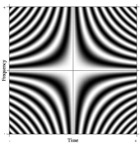
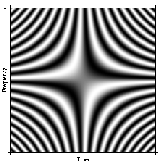
In the limit: The Fourier operator

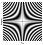Real part of Fourier operator

Imaginary part of Fourier operator

If we make a very large matrix with complex exponentials in the rows (i.e., cosine real parts and sine imaginary parts), and increase the resolution without bound, we approach the kernel of the Fredholm integral equation of the 2nd kind, namely the Fourier operator that defines the continuous Fourier transform. A rectangular portion of this continuous Fourier operator can be displayed as an image, analogous to the DFT matrix, as shown at right, where greyscale pixel value denotes numerical quantity.

References

• The Transform and Data Compression Handbook by P. C. Yip, K. Ramamohan Rao - See chapter 2 for a treatment of the DFT based largely on the DFT matrix

External links

• Fourier Operator and Decimation In Time (DIT)