Comparative statics

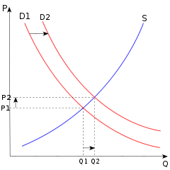In this graph, comparative statics shows an increase in demand causing a rise in price and quantity. Comparing two equilibrium states, comparative statics doesn't describe how the increases actually occur.

In economics, comparative statics is the comparison of two different economic outcomes, before and after a change in some underlying exogenous parameter.^[1]

As a study of statics it compares two different equilibrium states, after the process of adjustment (if any). It does not study the motion towards equilibrium, nor the process of the change itself.

Comparative statics is commonly used to study changes in supply and demand when analyzing a single market, and to study changes in monetary or fiscal policy when analyzing the whole economy. The term 'comparative statics' itself is more commonly used in relation to microeconomics (including general equilibrium analysis) than to macroeconomics. Comparative statics was formalized by John R. Hicks (1939) and Paul A. Samuelson (1947) (Kehoe, 1987, p. 517) but was presented graphically from at least the 1870s.^[2]

For models of stable equilibrium rates of change, such as the neoclassical growth model, comparative dynamics is the counterpart of comparative statics (Eatwell, 1987).

Linear approximation

Comparative statics results are usually derived by using the implicit function theorem to calculate a linear approximation to the system of equations that defines the equilibrium, under the assumption that the equilibrium is stable. That is, if we consider a sufficiently small change in some exogenous parameter, we can calculate how each endogenous variable changes using only the first derivatives of the terms that appear in the equilibrium equations.

For example, suppose the equilibrium value of some endogenous variable x is determined by the following equation:

f(x,a) = 0

where a is an exogenous parameter. Then, to a first-order approximation, the change in x caused by a small change in a must satisfy:

Bdx + Cda = 0

Here dx and da represent the changes in x and a, respectively, while B and C are the partial derivatives of f with respect to x and a (evaluated at the initial values of x and a), respectively. Equivalently, we can write the change in x as:

dx = − B ^{− 1}Cda.

The factor of proportionality − B ^{− 1}C is sometimes called the multiplier of a on x.

Many equations and unknowns

All the equations above remain true in the case of a system of n equations in n unknowns. In other words, suppose f(x,a) = 0 represents a system of n equations involving the vector of n unknowns x, and the vector of m given parameters a. If we make a sufficiently small change da in the parameters, then the resulting change in the endogenous variables can be approximated arbitrarily well by dx = − B ^{− 1}Cda. In this case, B represents the n-by-n matrix of partial derivatives of the functions f with respect to the variables x, and C represents the n-by-m matrix of partial derivatives of the functions f with respect to the parameters a. (The derivatives in B and C are evaluated at the initial values of x and a.)

Stability

The assumption that the equilibrium is stable matters for two reasons. First, if the equilibrium were unstable, a small parameter change might cause a large jump in the value of x, invalidating the use of a linear approximation. Moreover, Paul A. Samuelson's correspondence principle states that stability of equilibrium has testable implications about the comparative static effects. In other words, knowing that the equilibrium is stable may help us predict whether the coefficient B ^{− 1}C is positive or negative.

An example of the role of the stability assumption

Suppose that the quantities demanded and supplied of a product are determined by the following equations:

Q^d(P) = a + bP

Q^s(P) = c + gP

where Q^d is the quantity demanded, Q^s is the quantity supplied, P is the price, a and c are intercept parameters determined by exogenous influences on demand and supply respectively, b < 0 is the reciprocal of the slope of the demand curve, and g is the reciprocal of the slope of the supply curve; g > 0 if the supply curve is upward sloped, g = 0 if the supply curve is vertical, and g < 0 if the supply curve is backward-bending. If we equate quantity supplied with quantity demanded to find the equilibrium price P^eqb, we find that

$P^{eqb}=\frac{a-c}{g-b}.$

This means that the equilibrium price depends positively on the demand intercept if g – b > 0, but depends negatively on it if g – b < 0. Which of these possibilities is relevant? In fact, starting from an initial static equilibrium and then changing a, the new equilibrium is relevant only if the market actually goes to that new equilibrium. Suppose that price adjustments in the market occur according to

$\frac{dP}{dt}=\lambda (Q^{d}(P) - Q^{s}(P))$

where λ > 0 is the speed of adjustment parameter and $\frac{dP}{dt}$ is the time derivative of the price — that is, it denotes how fast and in what direction the price changes. By stability theory, P will converge to its equilibrium value if and only if the derivative $\frac{d(dP/dt)}{dP}$ is negative. This derivative is given by

$\frac{d(dP/dt)}{dP} = - \lambda(-b+g).$

This is negative if and only if g – b > 0, in which case the demand intercept parameter a positively influences the price. So we can say that while the direction of effect of the demand intercept on the equilibrium price is ambiguous when all we know is that the reciprocal of the supply curve's slope, g, is negative, in the only relevant case (in which the price actually goes to its new equilibrium value) an increase in the demand intercept increases the price. Note that this case, with g – b > 0, is the case in which the supply curve, if negatively sloped, is steeper than the demand curve.

Comparative statics without constraints

Suppose p(x;q) is a smooth and strictly concave objective function where x is a vector of n endogenous variables and q is a vector of m exogenous parameters. Consider the unconstrained optimization problem x ^* (q) = arg max p(x;q). Let f(x;q) = D_xp(x;q), the n by n matrix of first partial derivatives of p(x;q) with respect to its first n arguments x_i,...,x_n. The maximizer x ^* (q) is defined by the first order condition f(x ^* (q);q) = 0.

Comparative statics asks how this maximizer changes in response to changes in the m parameters. The aim is to find $\partial x^*_i/ \partial q_j, i=1,...,n, j=1,...,m$.

The strict concavity of the objective function implies that the Jacobian of f, which is exactly the matrix of second partial derivatives of p with respect to the endogenous variables, is nonsingular. By the implicit function theorem, then, x ^* (q) may be viewed locally as a continuously differentiable function, and the local response of x ^* (q) to small changes in q is given by

D_qx ^* (q) = − [D_xf(x * (q);q] ^{− 1}D_qf(x ^* (q);q).

Applying the chain rule and first order condition,

$D_qp(x^*(q),q)=D_qp(x;q)|_{x=x^*(q)}.$

(See Envelope theorem).

Application for profit maximization

Suppose a firm produces n goods in quantities x₁,...,x_n. The firm's profit is a function p of x₁,...,x_n and of m exogenous parameters q₁,...,q_m which may represent, for instance, various tax rates. Provided the profit function satisfies the smoothness and concavity requirements, the comparative statics method above describes the changes in the firms profit due to small changes in the tax rates.

Comparative statics with constraints

A generalization of the above method allows the optimization problem to include a set of constraints. This leads to the general envelope theorem. Applications include determining changes in Marshallian demand in response to changes in price or wage.

Monotone comparative statics

One limitation of comparative statics using the implicit function theorem is that results are valid only in a (potentially very small) neighborhood of the optimum. Another limitation is that results are cardinal rather than ordinal; that is, results are not robust to a monotone transformation of the objective function. For economic applications, ordinal results are preferred. In particular, monotone strictly increasing transformations of a utility function represent the same preference relation.

Paul Milgrom and Chris Shannon developed a theory and method for comparative statics analysis using only conditions that are ordinal. ^[3] The method uses lattice theory and introduces the notions of quasi-supermodularity and the single-crossing condition. The central theorem of monotone comparative statics is:

Suppose $p : R^n \times R^m \rightarrow R$ and let x ^* (q) = arg max p(x;q). Suppose $|x^*(q)=1| \forall q$, 'p' is quasi-supermodular in 'x' and satisfies the single-crossing property. Then

$q\geq r \implies x^*(q) \geq x^*(r).$

See also

• Microeconomics
• Model (economics)
• Qualitative economics

Notes

1. ^ (Mas-Colell, Whinston, and Green, 1995, p. 24; Silberberg and Suen, 2000)
2. ^ Fleeming Jenkin (1870), "The Graphical Representation of the Laws of Supply and Demand, and their Application to Labour," in Alexander Grant, Recess Studies and (1872), "On the principles which regulate the incidence of taxes," Proceedings of Royal Society of Edinburgh 1871-2, pp. 618-30., also in Papers, Literary, Scientific, &c, v. 2 {1887), ed. S.C. Colvin and J.A. Ewing via scroll to chapter links.
3. ^ Milgrom and Shannon. "Monotone Comparative Statics" (1994). Econometrica, Vol. 62 Issue 1, pp. 157-180, http://www.core.ucl.ac.be/clsAmir/MS1994.pdf.

References

• John Eatwell et al., ed. (1987). "Comparative dynamics," The New Palgrave: A Dictionary of Economics, v. 1, p. 517.
• John R. Hicks (1939). Value and Capital.
• Timothy J. Kehoe, 1987. "Comparative statics," The New Palgrave: A Dictionary of Economics, v. 1, pp. 517-20.
• Andreu Mas-Colell, Michael D. Whinston, and Jerry R. Green, 1995. Microeconomic Theory.
• Paul A. Samuelson (1947). Foundations of Economic Analysis.
• Eugene Silberberg and Wing Suen, 2000. The Structure of Economics: A Mathematical Analysis, 3rd edition.

External links

• San Jose State University Economics Department - Comparative Statics Analysis
• AmosWeb Glossary
• IFCI Risk Institute Glossary (from the American Stock Exchange glossary) [1]