Maze generation algorithm

Maze generation algorithms are automated methods for the creation of mazes.

This maze generated by modified version of Prim's algorithm, below.

Graph theory based methods

A maze can be generated by starting with a predetermined arrangement of cells (most commonly a rectangular grid but other arrangements are possible) with wall sites between them. This predetermined arrangement can be considered as a connected graph with the edges representing possible wall sites and the nodes representing cells. The purpose of the maze generation algorithm can then be considered to be making a subgraph where it is challenging to find a route between two particular nodes.

If the subgraph is not connected, then there are regions of the graph that are wasted because they do not contribute to the search space. If the graph contains loops, then there may be multiple paths between the chosen nodes. Because of this, maze generation is often approached as generating a random spanning tree. Loops which can confound naive maze solvers may be introduced by adding random edges to the result during the course of the algorithm.

Depth-first search

An animation of generating a 30 by 20 maze using depth-first search.

This algorithm is a randomized version of the depth-first search algorithm. Frequently implemented with a stack, this approach is one of the simplest ways to generate a maze using a computer. Consider the space for a maze being a large grid of cells (like a large chess board), each cell starting with four walls. Starting from a random cell, the computer then selects a random neighbouring cell that has not yet been visited. The computer removes the 'wall' between the two cells and adds the new cell to a stack (this is analogous to drawing the line on the floor). The computer continues this process, with a cell that has no unvisited neighbours being considered a dead-end. When at a dead-end it backtracks through the path until it reaches a cell with an unvisited neighbour, continuing the path generation by visiting this new, unvisited cell (creating a new junction). This process continues until every cell has been visited, causing the computer to backtrack all the way back to the beginning cell. This approach guarantees that the maze space is completely visited.

As stated, the algorithm is very simple and does not produce overly-complex mazes. More specific refinements to the algorithm can help to generate mazes that are harder to solve.

1. Start at a particular cell and call it the "exit."
2. Mark the current cell as visited, and get a list of its neighbors. For each neighbor, starting with a randomly selected neighbor:
   1. If that neighbor hasn't been visited, remove the wall between this cell and that neighbor, and then recurse with that neighbor as the current cell.

As given above this algorithm involves deep recursion which may cause stack overflow issues on some computer architectures. The algorithm can be rearranged into a loop by storing backtracking information in the maze itself. This also provides a quick way to display a solution, by starting at any given point and backtracking to the exit.

Mazes generated with a depth-first search have a low branching factor and contain many long corridors, which makes depth-first a good algorithm for generating mazes in video games. Randomly removing a number of walls after creating a DFS-maze can make its corridors less narrow, which can be suitable in situations where the difficulty of solving the maze is not of importance. This too can be favorable in video games.

In mazes generated by that algorithm, it will typically be relatively easy to find the way to the square that was first picked at the beginning of the algorithm, since most paths lead to or from there, but it is hard to find the way out.

Recursive backtracker

The depth-first search algorithm of maze generation is frequently implemented using backtracking:

1. Make the initial cell the current cell and mark it as visited
2. While there are unvisited cells
   1. If the current cell has any neighbours which have not been visited
      1. Choose randomly one of the unvisited neighbours
      2. Push the chosen cell to the stack
      3. Remove the wall between the current cell and the chosen cell
      4. Make the chosen cell the current cell and mark it as visited
   2. Else
      1. Pop a cell from the stack
      2. Make it the current cell

Randomized Kruskal's algorithm

This algorithm is a randomized version of Kruskal's algorithm.

1. Create a list of all walls, and create a set for each cell, each containing just that one cell.
2. For each wall, in some random order:
   1. If the cells divided by this wall belong to distinct sets:
      1. Remove the current wall.
      2. Join the sets of the formerly divided cells.

There are several data structures that can be used to model the sets of cells. An efficient implementation using a disjoint-set data structure can perform each union and find operation on two sets in nearly-constant amortized time (specifically, O(α(V)) time; α(x) < 5 for any plausible value of x), so the running time of this algorithm is essentially proportional to the number of walls available to the maze.

It matters little whether the list of walls is initially randomized or if a wall is randomly chosen from a nonrandom list, either way is just as easy to code.

Because the effect of this algorithm is to produce a minimal spanning tree from a graph with equally-weighted edges, it tends to produce regular patterns which are fairly easy to solve.

Randomized Prim's algorithm

An animation of generating a 30 by 20 maze using Prim's algorithm.

This algorithm is a randomized version of Prim's algorithm.

1. Start with a grid full of walls.
2. Pick a cell, mark it as part of the maze. Add the walls of the cell to the wall list.
3. While there are walls in the list:
   1. Pick a random wall from the list. If the cell on the opposite side isn't in the maze yet:
      1. Make the wall a passage and mark the cell on the opposite side as part of the maze.
      2. Add the neighboring walls of the cell to the wall list.
   2. If the cell on the opposite side already was in the maze, remove it from the list.

Like the depth-first algorithm, it will usually be relatively easy to find the way to the starting cell, but hard to find the way anywhere else.

Note that simply running classical Prim's on a graph with random weights would create mazes stylistically identical to Kruskal's, because they are both minimal spanning tree algorithms. Instead, this algorithm introduces stylistic variation because the edges closer to the starting point have a lower effective weight.

Modified version

Although the classical Prim's algorithm keeps a list of edges, for maze generation we could instead maintain a list of adjacent cells. If the randomly chosen cell has multiple edges that connect it to the existing maze, select one of these edges at random. This will tend to branch slightly more than the edge-based version above.

Recursive division method

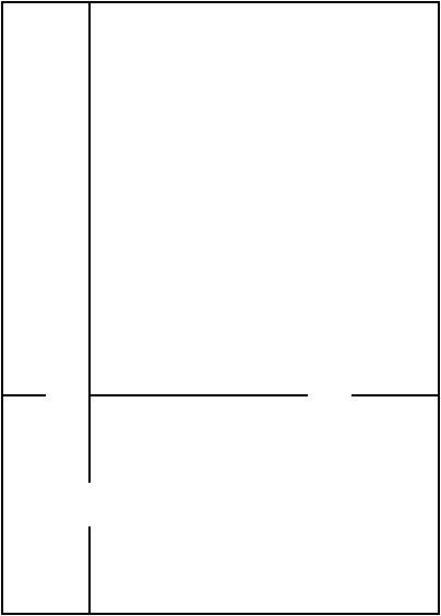
Illustration of Recursive Division

original chamber	division by two walls	holes in walls	continue subdividing...	completed

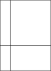
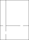
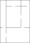
Mazes can be created with recursive division, an algorithm which works as follows: Begin with the maze's space with no walls. Call this a chamber. Divide the chamber with a randomly positioned wall (or multiple walls) where each wall contains a randomly positioned passage opening within it. Then recursively repeat the process on the subchambers until all chambers are minimum sized. This method results in mazes with long straight walls crossing their space, making it easier to see which areas to avoid.

For example, in a rectangular maze, build at random points two walls that are perpendicular to each other. These two walls divide the large chamber into four smaller chambers separated by four walls. Choose three of the four walls at random, and open a one cell-wide hole at a random point in each of the three. Continue in this manner recursively, until every chamber has a width of one cell in either of the two directions.

Simple algorithms

3D version of Prim's algorithm. Vertical layers are labeled 1 through 4 from bottom to top. Stairs up are indicated with "/"; stairs down with "\", and stairs up-and-down with "x". Source code is included with the image description.

Other algorithms exist that require only enough memory to store one line of a 2D maze or one plane of a 3D maze. They prevent loops by storing which cells in the current line are connected through cells in the previous lines, and never remove walls between any two cells already connected.

Most maze generation algorithms require maintaining relationships between cells within it, to ensure the end result will be solvable. Valid simply connected mazes can however be generated by focusing on each cell independently. A binary tree maze is a standard orthogonal maze where each cell always has a passage leading up or leading left, but never both. To create a binary tree maze, for each cell flip a coin to decide whether to add a passage leading up or left. Always pick the same direction for cells on the boundary, and the end result will be a valid simply connected maze that looks like a binary tree, with the upper left corner its root.

A related form of flipping a coin for each cell is to create an image using a random mix of forward slash and backslash characters. This doesn't generate a valid simply connected maze, but rather a selection of closed loops and unicursal passages. (The manual for the Commodore 64 presents a BASIC program using this algorithm, but using PETSCII diagonal line graphic characters instead for a smoother graphic appearance.)

Cellular automata algorithms

Certain types of cellular automata can be used to generate mazes. ^[1] Two well-known such cellular automata, Maze and Mazetric, have rulestrings 12345/3 and 1234/3.^[1] In the former, this means that cells survive from one generation to the next if they have at least one and at most five neighbours. In the latter, this means that cells survive if they have one to four neighbours. If a cell has exactly three neighbours, it is born. It is similar to Conway's Game of Life in that patterns that do not have a living cell adjacent to 1, 4, or 5 other living cells in any generation will behave identically to it.^[1] However, for large patterns, it behaves very differently.^[1]

For a random starting pattern, these maze-generating cellular automata will evolve into complex mazes with well-defined walls outlining corridors. Mazecetric, which has the rule 1234/3 has a tendency to generate longer and straighter corridors compared with Maze, with the rule 12345/3.^[1] Since these cellular automaton rules are deterministic, each maze generated is uniquely determined by its random starting pattern. This is a significant drawback since the mazes tend to be relatively predictable.

Like some of the graph-theory based methods described above, these cellular automata typically generate mazes from a single starting pattern; hence it will usually be relatively easy to find the way to the starting cell, but harder to find the way anywhere else.

Python code example

import numpy as np
from numpy.random import random_integers as rnd
import matplotlib.pyplot as plt
 
def maze(width=81, height=51, complexity=.75, density =.75):
    # Only odd shapes
    shape = ((height//2)*2+1, (width//2)*2+1)
    # Adjust complexity and density relative to maze size
    complexity = int(complexity*(5*(shape[0]+shape[1])))
    density    = int(density*(shape[0]//2*shape[1]//2))
    # Build actual maze
    Z = np.zeros(shape, dtype=bool)
    # Fill borders
    Z[0,:] = Z[-1,:] = 1
    Z[:,0] = Z[:,-1] = 1
    # Make isles
    for i in range(density):
        x, y = rnd(0,shape[1]//2)*2, rnd(0,shape[0]//2)*2
        Z[y,x] = 1
        for j in range(complexity):
            neighbours = []
            if x > 1:           neighbours.append( (y,x-2) )
            if x < shape[1]-2:  neighbours.append( (y,x+2) )
            if y > 1:           neighbours.append( (y-2,x) )
            if y < shape[0]-2:  neighbours.append( (y+2,x) )
            if len(neighbours):
                y_,x_ = neighbours[rnd(0,len(neighbours)-1)]
                if Z[y_,x_] == 0:
                    Z[y_,x_] = 1
                    Z[y_+(y-y_)//2, x_+(x-x_)//2] = 1
                    x, y = x_, y_
    return Z
 
plt.figure(figsize=(10,5))
plt.imshow(maze(80,40),cmap=plt.cm.binary,interpolation='nearest')
plt.xticks([]),plt.yticks([])
plt.show()

References

1. ^ ^{a b c d e} Nathaniel Johnston et al (21 August 2010). "Maze - LifeWiki". LifeWiki. http://www.conwaylife.com/wiki/index.php?title=Maze. Retrieved 1 March 2011. 

See also

• Mazes
• Maze solving algorithm

External links

• Think Labyrinth: Maze algorithms (details on these and other maze generation algorithms)
• Explanation of an Obfuscated C maze algorithm (a program to generate mazes line-by-line, obfuscated in a single physical line of code)
• Maze generation and solving Java applet
• Maze generating Java applets with source code.
• Maze Generation - Master's Thesis (Java Applet enabling users to have a maze created using various algorithms and human solving of mazes)
• Create Your Own Mazes
• Collection of maze generation code in different languages in Rosetta Code
• Maze Generation Using JavaScript