Cellular model

Part of the Cell Cycle

Creating a cellular model has been a particularly challenging task of systems biology and mathematical biology. It involves developing efficient algorithms, data structures, visualization and communication tools to orchestrate the integration of large quantities of biological data with the goal of computer modeling.

It is also directly associated with bioinformatics, computational biology and Artificial life.

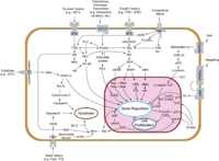
It involves the use of computer simulations of the many cellular subsystems such as the networks of metabolites and enzymes which comprise metabolism, signal transduction pathways and gene regulatory networks to both analyze and visualize the complex connections of these cellular processes.

The complex network of biochemical reaction/transport processes and their spatial organization make the development of a predictive model of a living cell a grand challenge for the 21st century.

Overview

The eukaryotic cell cycle is very complex and is one of the most studied topics, since its misregulation leads to cancers. It is possibly a good example of a mathematical model as it deals with simple calculus but gives valid results. Two research groups ^[1][2] have produced several models of the cell cycle simulating several organisms. They have recently produced a generic eukaryotic cell cycle model which can represent a particular eukaryote depending on the values of the parameters, demonstrating that the idiosyncrasies of the individual cell cycles are due to different protein concentrations and affinities, while the underlying mechanisms are conserved (Csikasz-Nagy et al., 2006).
By means of a system of ordinary differential equations these models show the change in time (dynamical system) of the protein inside a single typical cell; this type of model is called a deterministic process (whereas a model describing a statistical distribution of protein concentrations in a population of cells is called a stochastic process).
To obtain these equations an iterative series of steps must be done: first the several models and observations are combined to form a consensus diagram and the appropriate kinetic laws are chosen to write the differential equations, such as rate kinetics for stoichiometric reactions, Michaelis-Menten kinetics for enzyme substrate reactions and Goldbeter–Koshland kinetics for ultrasensitive transcription factors, afterwards the parameters of the equations (rate constants, enzyme efficiency coefficients and Michealis constants) must be fitted to match observations; when they cannot be fitted the kinetic equation is revised and when that is not possible the wiring diagram is modified. The parameters are fitted and validated using observations of both wild type and mutants, such as protein half-life and cell size.
In order to fit the parameters the differential equations need to be studied. This can be done either by simulation or by analysis.
In a simulation, given a starting vector (list of the values of the variables), the progression of the system is calculated by solving the equations at each time-frame in small increments.
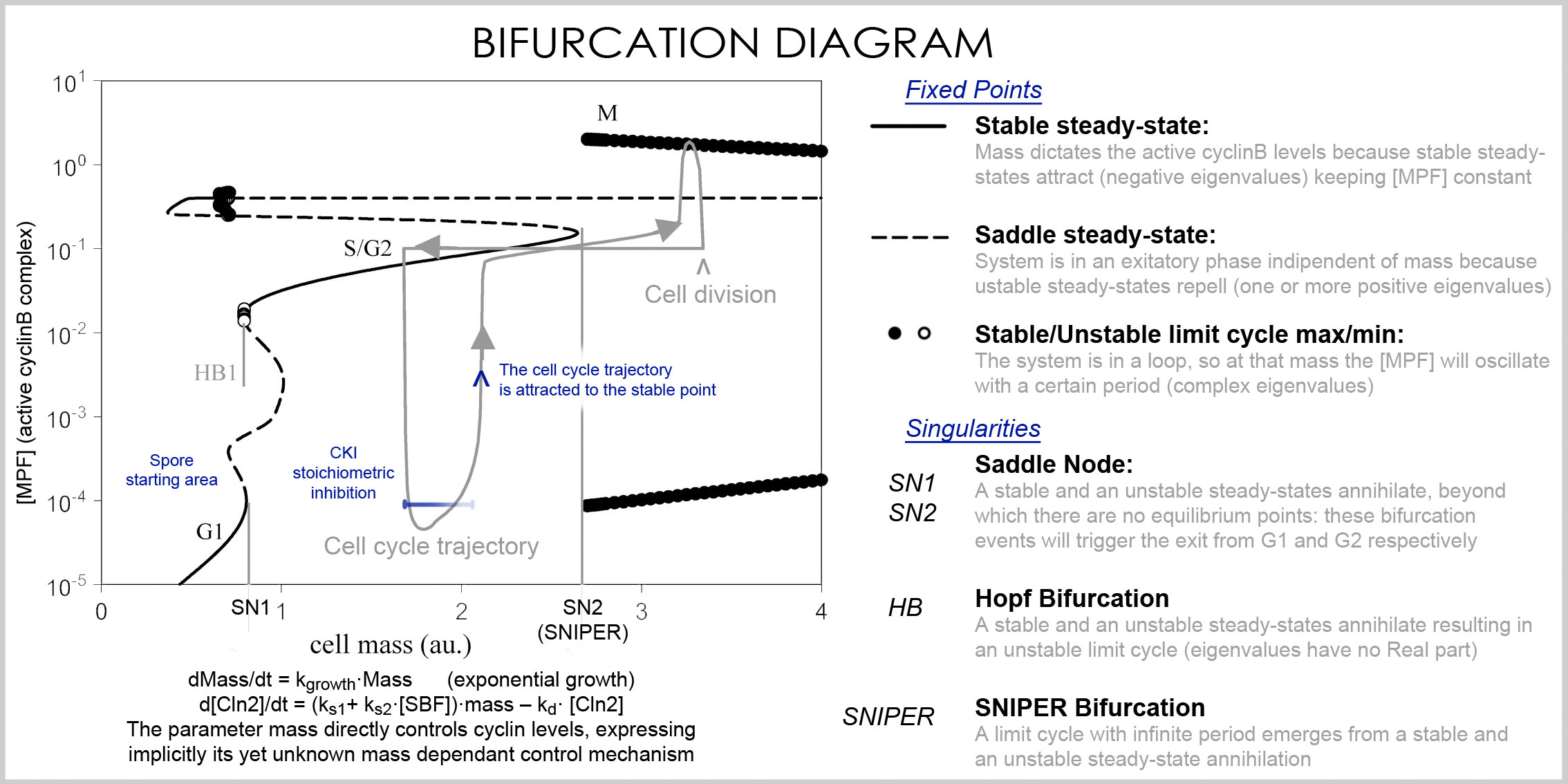
In analysis, the proprieties of the equations are used to investigate the behavior of the system depending of the values of the parameters and variables. A system of differential equations can be represented as a vector field, where each vector described the change (in concentration of two or more protein) determining where and how fast the trajectory (simulation) is heading. Vector fields can have several special points: a stable point, called a sink, that attracts in all directions (forcing the concentrations to be at a certain value), an unstable point, either a source or a saddle point which repels (forcing the concentrations to change away from a certain value), and a limit cycle, a closed trajectory towards which several trajectories spiral towards (making the concentrations oscillate).
A better representation which can handle the large number of variables and parameters is called a bifurcation diagram (bifurcation theory): the presence of these special steady-state points at certain values of a parameter (e.g. mass) is represented by a point and once the parameter passes a certain value, a qualitative change occurs, called a bifurcation, in which the nature of the space changes, with profound consequences for the protein concentrations: the cell cycle has phases (partially corresponding to G1 and G2) in which mass, via a stable point, controls cyclin levels, and phases (S and M phases) in which the concentrations change independently, but once the phase has changed at a bifurcation event (cell cycle checkpoint), the system cannot go back to the previous levels since at the current mass the vector field is profoundly different and the mass cannot be reversed back through the bifurcation event, making a checkpoint irreversible. In particular the S and M checkpoints are regulated by means of special bifurcations called a Hopf bifurcation and an infinite period bifurcation.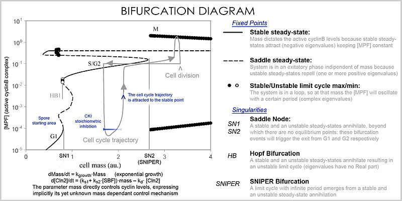

Molecular level simulations

E-Cell Project aims "to make precise whole cell simulation at the molecular level possible".^[3]

Projects

Multiple projects are in progress.^[4]

• Karyote - Indiana University
• E-Cell Project
• Virtual Cell - University of Connecticut Health Center
• Silicon Cell

See also

• Biological data visualization
• Molecular modeling software
• Membrane computing is the task of modeling specifically a cell membrane.
• Biochemical Switches in the Cell Cycle
• Masaru Tomita

References

1. ^ "The JJ Tyson Lab". Virginia Tech. http://mpf.biol.vt.edu/lab_website/. Retrieved 2011-07-20. 
2. ^ "The Molecular Network Dynamics Research Group". Budapest University of Technology and Economics. http://www.cellcycle.bme.hu/. 
3. ^ http://www.e-cell.org/ecell/
4. ^ http://www.nature.com/naturejobs/2002/020627/full/nj6892-04a.html