Compartmental models in epidemiology

In order to model the progress of an epidemic in a large population, comprising many different individuals in various fields, the population diversity must be reduced to a few key characteristics which are relevant to the infection under consideration. For example, for most common childhood diseases that confer long-lasting immunity it makes sense to divide the population into those who are susceptible to the disease, those who are infected and those who have recovered and are immune. These subdivisions of the population are called compartments.

The SIR model

Standard convention labels these three compartments S (for susceptible), I (for infectious) and R (for recovered). Therefore, this model is called the SIR model.

This is a good and simple model for many infectious diseases including measles, mumps and rubella.

The letters also represent the number of people in each compartment at a particular time. To indicate that the numbers might vary over time (even if the total population size remains constant), we make the precise numbers a function of t (time): S(t), I(t) and R(t). For a specific disease in a specific population, these functions may be worked out in order to predict possible outbreaks and bring them under control.

The SIR model is dynamic in three senses

As implied by the variable function of t, the model is dynamic in that the numbers in each compartment may fluctuate over time. The importance of this dynamic aspect is most obvious in an endemic disease with a short infectious period, such as measles in the UK prior to the introduction of a vaccine in 1968. Such diseases tend to occur in cycles of outbreaks due to the variation in number of susceptibles (S(t)) over time. During an epidemic, the number of susceptible individuals falls rapidly as more of them are infected and thus enter the infectious and recovered compartments. The disease cannot break out again until the number of susceptibles has built back up as a result of babies being born into the susceptible compartment.

Blue=Susceptible, Green=Infected, and Red=Recovered

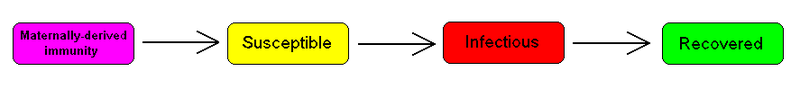
Each member of the population typically progresses from susceptible to infectious to recovered. This can be shown as a flow diagram in which the boxes represent the different compartments and the arrows the transition between compartments.

Transition rates

For the full specification of the model, the arrows should be labeled with the transition rates between compartments.

Between S and I, the transition rate is β I, where β is the contact rate, which -roughly speaking - takes into the account the probability of getting the disease in a contact between a susceptible and an infectious subject.

Between I and R, the transition rate is ν (simply the rate of recovery). If the duration of the infection is denoted D, then ν = 1/D, since an individual experiences one recovery in D units of time.

It is important to stress that here we assume that the permanence of each single subject in the epidemic states is a random variable with exponential distribution. More complex and realistic distributions (such as Erlang distributions) can be equally used with few modifications.

Bio-mathematical deterministic treatment of the SIR model

The SIR model without vital dynamics

A single epidemic outbreak is usually far more rapid than the vital dynamics of a population, thus, if the aim is to study the immediate consequences of a single epidemic, one may neglect the birth-death processes. In this case the SIR system described above can be expressed by the following set of ordinary differential equations:

$\frac{dS}{dt} = - \beta I S$

$\frac{dI}{dt} = \beta I S - \nu I$

$\frac{dR}{dt} = \nu I$

This model was for the first time proposed by O. Kermack and Anderson Gray McKendrick, who had worked with the Nobel Laureate Ronald Ross.

This system is non-linear, and does not admit a generic analytic solution. Nevertheless, significant results can be derived analytically.

Firstly note that from:

$\frac{dS}{dt} + \frac{dI}{dt} + \frac{dR}{dt} = 0$

it follows that:

S(t) + I(t) + R(t) = Constant = N

expressing in mathematical terms the constancy of population N. Note that the above relationship implies that one can study the equation for only two of the three variables.

Secondly, we note that the dynamics of the infectious class depends on the following ratio:

$R_0 = N\frac{\beta}{\nu}$

the so-called basic reproduction number (also called basic reproduction ratio). This ratio is derived as the expected number of new infections from a single infection in a population where all subjects are susceptible ^[1] .^[2]

By dividing the first differential equation by the third, separating the variables and integrating we get

$S(t) = S(0) e^{-R_0(R(t) - R(0))}$

(where S(0) and R(0) are the initial numbers of, respectively, susceptible and removed subjects). Thus, in the limit $t \rightarrow +\infty$, the proportion of recovered individuals obeys the transcendental equation

$R_{\infty} = 1 - S(0)e^{-R_0(R_{\infty} - R(0))}$

Consideration of this equation shows that generically, at the end of an epidemic, not all individuals have recovered, so some must remain susceptible. This means that the end of an epidemic is caused by the decline in the number of infected individuals rather than an absolute lack of susceptible subjects. The role of the basic reproduction number is extremely important. In fact, upon rewriting the equation for infectious individuals as follows:

$\frac{dI}{dt} = (R_0 S - 1) \nu I$

it yields that if:

$R_{0} > \frac{1}{S(0)} ,$

then:

$\frac{dI}{dt}(0) >0 ,$

i.e. there will be a proper epidemic outbreak with an increase of the number of the infectious (which can reach a considerable fraction of the population). On the contrary, if

$R_{0} < \frac{1}{S(0)} ,$

then

$\frac{dI}{dt}(0) <0 ,$

i.e. independently from the initial size of the susceptible population the disease can never cause a proper epidemic outbreak. As a consequence, it is clear that the basic reproduction number is extremely important.

The force of infection

Note that in the above model the function:

F = βI,

models the transition rate from the compartment of susceptible individuals to the compartment of infectious individuals, so that it is called the force of infection. However, for large classes of communicable diseases it is more realistic to consider a force of infection that does not depend on the absolute number of infectious subjects, but on their fraction (with respect to the total constant population N):

$F = \beta \frac{I}{N} .$

Capasso and, afterwards, other authors have proposed nonlinear forces of infection to model more realistically the contagion process.

The SIR model with vital dynamics and constant population

Considering a population characterized by a death rate μ and birth rate equal to the death rate, and where a communicable disease is spreading. The model is:

$\frac{dS}{dt} = \mu N - \mu S - \beta \frac{I}{N} S$

$\frac{dI}{dt} = \beta \frac{I}{N} S - (\nu +\mu ) I$

$\frac{dR}{dt} = \nu I - \mu R$

for which it holds:

S + I + R = N.

Also in this case we may define a basic reproduction number :

$R_0 = \frac{ \beta }{\mu+\nu},$

which has threshold properties. In fact, independently from biologically meaningful initial values:

$\left(S(0),I(0),R(0)\right) \in \left\{(S,I,R)\in [0,N]^3 : S \ge 0, I\ge 0, R\ge 0, S+I+R = N \right\}$

one can show that:

$R_0 \le 1 \Rightarrow \lim_{t \rightarrow +\infty} \left(S(t),I(t),R(t)\right) = DFE = \left(N,0,0\right)$

$R_0 > 1 , I(0)> 0 \Rightarrow \lim_{t \rightarrow +\infty} \left(S(t),I(t),R(t)\right) = EE = \left(\frac{N}{R_0},\frac{\mu}{\beta}\left(R_0-1\right)N,\frac{\nu}{\beta} \left(R_0-1\right)N\right).$

The point DFE is called the disease free equilibrium, whereas the point EE is called the Endemic Equilibrium. Since, with heuristic arguments, one may show that R₀ may be read as the average number of infections caused by a single infectious subject in a wholly susceptible population, the above relationship biologically means that if this number is less or equal than one the disease get extinct, whereas if this number is greater than one the disease will remain permanently endemic in the population.

Variable contact rates and pluriannual or chaotic epidemics

It is well known that the probability of getting a disease is not constant in the time. It is common experience that some diseases are more frequently present in the winter, and other in the summer in dependence of the weather. Moreover, for childhood diseases, there is a strong influence of the school calendar, so that during the school holidays the probability of getting such a disease dramatically decreases. As a consequence, for many classes of diseases one should consider a force of infection with periodically ('seasonal') varying contact rate

$F = \beta(t) \frac{I}{N} , \beta(t+T)=\beta(t)$

with period T equal to one year.

Thus, our model becomes

$\frac{dS}{dt} = \mu N - \mu S - \beta(t) \frac{I}{N} S$

$\frac{dI}{dt} = \beta(t) \frac{I}{N} S - (\nu +\mu ) I$

(the dynamics of recovered easily follows from R = N − S − I), idest a nonlinear set of differential equations with periodically varying parameters. It is well known that this class of dynamical systems may undergo very interesting and complex phenomena of nonlinear parametric resonance. It is easy to see that if:

$\frac{1}{T} \int_{0}^{T}\frac{\beta(t)}{\mu+\nu}dt < 1 \Rightarrow \lim_{t \rightarrow +\infty} \left(S(t),I(t)\right) = DFE = \left(N,0\right),$

whereas if the integral is greater than one the disease will not die out and there may be such resonances. For example, considering the periodically varying contact rate as the 'input' of the system one has that the output is a periodic function whose period is a multiple of the period of the input. This allowed to give a contribution to explain the poly-annual (typically biennial) epidemic outbreaks of some infectious diseases as interplay between the period of the contact rate oscillations and the pseudo-period of the damped oscillations near the endemic equilibrium. Remarkably, in some cases the behavior may also be quasi-periodic or even chaotic.

Modelling mass vaccination programmes

Vaccinating the newborns

In presence of a communicable diseases, one of main tasks is that of eradicating it via prevention measures and, if possible, via the establishment of a mass vaccination program. Let us consider a disease for which the newborn are vaccinated (with a vaccine giving life-long immunity) at a rate $P \in (0,1)$:

$\frac{dS}{dt} = \mu N (1-P) - \mu S - \beta \frac{I}{N} S$

$\frac{dI}{dt} = \beta \frac{I}{N} S - (\mu+\nu) I$

$\frac{dV}{dt} = \mu N P - \mu V$

where V is the class of vaccinated subjects. It is immediate to show that:

$\lim_{t \rightarrow +\infty} V(t)= N P,$

thus we shall deal with the long term behavior of S and I, for which it holds that:

$R_0 (1-P) \le 1 \Rightarrow \lim_{t \rightarrow +\infty} \left(S(t),I(t)\right) = DFE = \left(N \left(1-P\right),0\right)$

$R_0 (1-P) > 1 , I(0)> 0 \Rightarrow \lim_{t \rightarrow +\infty} \left(S(t),I(t)\right) = EE = \left(\frac{N}{R_0(1-P)},N \left(R_0 (1-P)-1\right)\right).$

In other words if

$P \ge P^{*}= 1-\frac{1}{R_0}$

the vaccination program is successful in eradicating the disease, on the contrary it will remain endemic, although at lower levels than the case of absence of vaccinations. This means that the mathematical model suggests that for a disease whose basic reproduction number may be as high as 18 one should have to vaccinate 94.4% of newborns in order to eradicate the disease.

Vaccination and information

Modern societies are facing the challenge of "rational" exemption, i.e. the family's decision to not vaccinate children as a consequence of a "rational" comparison between the perceived risk from infection and that from getting damages from the vaccine. In order to assess whether this behavior is really rational, i.e. if it can equally lead to the eradication of the disease, one may simply assume that the vaccination rate is an increasing function of the number of infectious subjects:

$P=P(I),P^{\prime}(I)>0.$

In such a case the eradication condition becomes:

$P(0) \ge P^{*},$

i.e. the baseline vaccination rate should be greater than the "mandatory vaccination" threshold, which, in case of exemption, cannot hold. Thus, "rational" exemption might be myopic since it is based only on the current low incidence due to high vaccine coverage, instead taking into account future resurgence of infection due to coverage decline.

Vaccination of non newborns

In case there also are vaccinations of non newborn at a rate ρ the equation for the susceptible and vaccinated subject has to be modified as follows:

$\frac{dS}{dt} = \mu N (1-P) - \mu S - \rho S - \beta \frac{I}{N} S$

$\frac{dV}{dt} = \mu N P + \rho S - \mu V$

leading to the following eradication condition:

$P \ge 1- \left(1+\frac{\rho}{\mu}\right)\frac{1}{R_0}$

Pulse vaccination strategy

Pulse Vaccination Strategy is a vaccination policy consisting of periodical repetitions of 'impulsive' multi age-cohort vaccinations in a population, i.e. every T time units a constant fraction p of susceptible subjects is vaccinated in a relatively short (respect to the dynamics of the disease) time. This leads to the following impulsive differential equations for the susceptible and vaccinated subjects:

$\frac{dS}{dt} = \mu N - \mu S - \beta \frac{I}{N} S, S(n T^+) = (1-p) S(n T^-) n=0,1,2,\dots$

$\frac{dV}{dt} = - \mu V, V(n T^+) = V(n T^-) + p S(n T^-) n=0,1,2,\dots$

It is easy to see that by setting I=0 one obtains that the dynamics of the susceptible subjects is given by:

$S^*(t) = 1- \frac{p}{1-(1-p)E^{-\mu T}}E^{-\mu MOD(t,T)}$

and that the eradication condition is:

$R_0 \int_{0}^{T}{S^*(t)dt} < 1$

The SEIR model

For many important infections there is a significant period of time during which the individual has been infected but is not yet infectious themselves. During this latent period the individual is in compartment E (for exposed).

Assuming that the period of staying in the latent state is a random variable with exponential distribution with parameter a (i.e. the average latent period is a ^{− 1}), and also assuming the presence of vital dynamics with birth rate equal to death rate, we have the model:

$\frac{dS}{dt} = \mu N - \mu S - \beta \frac{I}{N} S$

$\frac{dE}{dt} = \beta \frac{I}{N} S - (\mu +a ) E$

$\frac{dI}{dt} = a E - (\nu +\mu ) I$

$\frac{dR}{dt} = \nu I - \mu R.$

Of course, we have that S + E + I + R = N.

For this model, the basic reproduction number is:

$R_0 = \frac{a}{\mu+a}\frac{\beta}{\mu+\nu}.$

Similarly to the SIR model, also in this case we have a Disease-Free-Equilibrium (N,0,0,0) and an Endemic Equilibrium EE, and one can show that, independently form biologically meaningful initial conditions

$\left(S(0),E(0),I(0),R(0)\right) \in \left\{(S,E,I,R)\in [0,N]^4 : S \ge 0, E \ge 0, I\ge 0, R\ge 0, S+E+I+R = N \right\}$

it holds that:

$R_0 \le 1 \Rightarrow \lim_{t \rightarrow +\infty} \left(S(t),E(t),I(t),R(t)\right) = DFE = \left(N,0,0,0\right)$

$R_0 > 1 , I(0)> 0 \Rightarrow \lim_{t \rightarrow +\infty} \left(S(t),E(t),I(t),R(t)\right) = EE.$

In case of periodically varying contact rate β(t) the condition for the global attractiveness of DFE is that the following linear system with periodic coefficients:

$\frac{dE_1}{dt} = \beta(t) I_1 - (\nu +a ) E_1$

$\frac{dI_1}{dt} = a E_1 - (\nu +\mu ) I_1$

is stable (i.e. it has its Floquet's eigenvalues inside the unit circle in the complex plane).

Elaborations on the basic SIR model

The MSIR model

For many infections, including measles, babies are not born into the susceptible compartment but are immune to the disease for the first few months of life due to protection from maternal antibodies (passed across the placenta or through colostrum). This added detail can be shown by including an M class (for maternally derived immunity) at the beginning of the model.

Carrier state

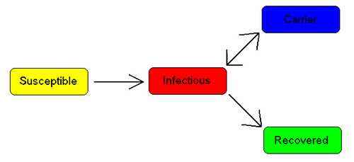
Some people who have had an infectious disease such as tuberculosis never completely recover and continue to carry the infection, whilst not suffering the disease themselves. They may then move back into the infectious compartment and suffer symptoms (as in tuberculosis) or they may continue to infect others in their carrier state, while not suffering symptoms. The most famous example of this is probably Mary Mallon, who infected 22 people with typhoid fever. The carrier compartment is labelled C.

The SIS model

Susceptibles and infected get equilibrated.

Some infections, for example the group of those responsible for the common cold, do not confer any long lasting immunity. Such infections do not have a recovered state and individuals become susceptible again after infection.

We have the model:

$\frac{dS}{dt} = - \beta S I + \gamma I$

$\frac{dI}{dt} = \beta S I - \gamma I$

Note that denoting with N the total population it holds that: $\frac{dS}{dt} + \frac{dI}{dt} = 0 \Rightarrow S(t)+I(t) = N$ it follows that:

$\frac{dI}{dt} = \left( \beta N - \gamma\right) I - \beta I^2$

i.e. the dynamics of infectious is ruled by a logistic equation, so that $\forall I(0) > 0$:

$\frac{\beta N}{\gamma} \le 1 \Rightarrow \lim_{t \rightarrow +\infty}I(t)=0$

$\frac{\beta N}{\gamma} > 1 \Rightarrow \lim_{t \rightarrow +\infty}I(t)=\frac{\beta N - \gamma}{\beta}$

The influence of age: age-structured models

Maybe "the most specific parameter of biological system is the age" (M. Iannelli), and, especially for some infectious diseases, it has a deep influence on the dynamics of its spreading in a population. Many of the parameters we have seen may depend on age, and especially the contact rate, which summarizes the 'infectious effectiveness' of contacts between susceptible and infectious subjects. This effectiveness has, thus, to take into account both the age of the infectious and the age of the susceptible. Epidemic models modeling the age structure of a population are very complex. In fact, they are infinite dimensional model since we have to deal with density through the ages of the epidemic classes s(t,a),i(t,a),r(t,a) (to limit ourselves to the susceptible-infectious-removed scheme) such that:

$S(t)=\int_0^{a_M}{s(t,a)da}$

$I(t)=\int_0^{a_M}{i(t,a)da}$

$R(t)=\int_0^{a_M}{r(t,a)da}$

(where $a_M \le +\infty$ is the maximum admissible age)and their dynamics is not described, as one might think, by "simple" partial differential equations, but by integro-differential equations:

$\partial_t s(t,a) + \partial_a s(t,a) = -\mu(a) s(a,t) - s(a,t)\int_{0}^{a_M}{k(a,a_1;t)i(a_1,t)da_1}$

$\partial_t i(t,a) + \partial_a i(t,a) = s(a,t)\int_{0}^{a_M}{k(a,a_1;t)i(a_1,t)da_1} -\mu(a) i(a,t) - \nu(a)i(a,t)$

$\partial_t r(t,a) + \partial_a r(t,a) = -\mu(a) r(a,t) + \nu(a)i(a,t)$

where:

$F(a,t,i(\cdot,\cdot))=\int_{0}^{a_M}{k(a,a_1;t)i(a_1,t)da_1}$

is the force of infection, which, of course, will depend, though the contact kernel k(a,a₁;t) on the interactions between the ages.

Complexity is added by the initial conditions for newborns (i.e. for a=0), that are straightforward for infectious and removed:

i(t,0) = r(t,0) = 0

but that are nonlocal for the density of susceptible newborns:

$s(t,0)= \int_{0}^{a_M}{\left(\varphi_s(a) s(a,t)+\varphi_i(a) i(a,t)+\varphi_r(a) r(a,t)\right) da}$

where φ_j(a),j = s,i,r are the fertilities of the adults.

Moreover, defining now the density of the total population n(t,a) = s(t,a) + i(t,a) + r(t,a) one obtains:

$\partial_t n(t,a) + \partial_a n(t,a) = -\mu(a) n(a,t)$

In the simplest case of equal fertilities in the three epidemic classes, we have that in oder to have demographic equilibrium the following necessary and sufficient condition linking the fertility φ(.) with the mortality μ(a) must hold:

$1 = \int_0^{a_M}{\varphi(a) \exp\left(- \int_0^a{\mu(q)dq} \right)da }$

and the demographic equilibrium is

$n^*(a)=C \exp\left(- \int_0^a{\mu(q)dq}\right),$

automatically ensuring the existence of the disease-free solution:

$DFS(a)= \left(n^*(a),0,0\right).$

A basic reproduction number can be calculated as the spectral radius of an appropriate functional operator.

Deterministic versus stochastic epidemic models

It is important to stress that the deterministic models presented here are valid only in case of sufficiently large populations. Moreover, even in case of large populations, as pointed out among the firsts by M. S. Bartlett, in some cases deterministic models should cautiously be used. For example in case of seasonally varying contact rates the number of infectious subjects may reduce to infinitesimal values, thus maybe invalidating some results that are obtained in the field of chaotic epidemics.

See also

• Mathematical modelling in epidemiology
• Modifiable Areal Unit Problem

References

1. ^ Bailey, Norman T. J. (1975). The mathematical theory of infectious diseases and its applications (2nd ed.). London: Griffin. ISBN 0-85264-231-8. 
2. ^ Sonia Altizer; Nunn, Charles (2006). Infectious diseases in primates: behavior, ecology and evolution. Oxford Series in Ecology and Evolution. Oxford [Oxfordshire]: Oxford University Press. ISBN 0-19-856585-2. 

Bibliography

• May, Robert Lewis; Anderson, Roy M. (1991). Infectious diseases of humans: dynamics and control. Oxford [Oxfordshire]: Oxford University Press. ISBN 0-19-854040-X. 

• V. Capasso, The Mathematical Structure of Epidemic Systems, Springer Verlag (1993)

• McKendrick AG (1925). "Applications of mathematics to medical problems". Proceedings of the Edinburgh Mathematical Society 44: 98–130. doi:10.1017/S0013091500034428. 
  Reprinted with commentary in Johnson, Norman L.; Kotz, Samuel (1992). Breakthroughs in statistics. 3. Berlin: Springer-Verlag. ISBN 0-387-94989-5. 

• Kermack WO, McKendrick AG (August 1, 1927). "A Contribution to the Mathematical Theory of Epidemics". Proc. R. Soc. Lond. A 115 (772): 700–721. doi:10.1098/rspa.1927.0118. 

• Kermack WO, McKendrick AG (October 1, 1932). "Contributions to the Mathematical Theory of Epidemics. II. The Problem of Endemicity". Proc. R. Soc. Lond. A 138 (834): 55–83. doi:10.1098/rspa.1932.0171. 

• Kermack WO, McKendrick AG (July 3, 1933). "Contributions to the Mathematical Theory of Epidemics. III. Further Studies of the Problem of Endemicity". Proc. R. Soc. Lond. A 141 (843): 94–122. doi:10.1098/rspa.1933.0106. 

• Bartlett MS (1957). "Measles periodicity and community size". J.r. Stat. Soc. A 120 (1): 48–70. doi:10.2307/2342553. JSTOR 2342553. 

• Hethcote H (1976). "Qualitative analyses of communicable disease models". Math. Biosci. 28 (3-4): 335–356. doi:10.1016/0025-5564(76)90132-2. http://www.math.uiowa.edu/~hethcote/PDFs/1976MathBiosci.pdf. 

• Olsen LF, Schaffer WM (August 1990). "Chaos versus noisy periodicity: alternative hypotheses for childhood epidemics". Science 249 (4968): 499–504. doi:10.1126/science.2382131. PMID 2382131. http://www.sciencemag.org/cgi/pmidlookup?view=long&pmid=2382131. 

• Inaba H (1990). "Threshold and stability results for an age-structured epidemic model". J Math Biol 28 (4): 411–34. PMID 2384720. 

• Agur Z, Cojocaru L, Mazor G, Anderson RM, Danon YL (December 1993). "Pulse mass measles vaccination across age cohorts". Proc. Natl. Acad. Sci. U.S.A. 90 (24): 11698–702. doi:10.1073/pnas.90.24.11698. PMC 48051. PMID 8265611. http://www.pubmedcentral.nih.gov/articlerender.fcgi?tool=pmcentrez&artid=48051. 

• Kuznetsov YA, Piccardi C (1994). "Bifurcation analysis pf periodic SEIR and SIR epidemic models". J Math Biol 32 (2): 109–21. doi:10.1007/BF00163027. PMID 8145028. 

• Li MY, Muldowney JS (February 1995). "Global stability for the SEIR model in epidemiology". Math Biosci 125 (2): 155–64. doi:10.1016/0025-5564(95)92756-5. PMID 7881192. http://linkinghub.elsevier.com/retrieve/pii/0025556495927565. 

• Nasell, I. (2002). "Measles outbreaks are not chaotic". In Blower, Sally; Castillo-Chávez, Carlos. Mathematical approaches for emerging and reemerging infectious diseases: an introduction. Berlin: Springer. pp. 85–115. ISBN 0-387-95354-X. 

• d'Onofrio A (2002). "Stability properties of pulse vaccination strategy in SEIR epidemic model". Math Biosci 179 (1): 57–72. doi:10.1016/S0025-5564(02)00095-0. PMID 12047921. 

• d'Onofrio A (2004). "Mixed pulse vaccination strategy in epidemic model with realistically distributed infectious and latent times". Applied Mathematics and Computation 151 (1): 181–7. doi:10.1016/S0096-3003(03)00331-X. 

• Reluga TC, Bauch CT, Galvani AP (December 2006). "Evolving public perceptions and stability in vaccine uptake". Math Biosci 204 (2): 185–98. doi:10.1016/j.mbs.2006.08.015. PMID 17056073. http://linkinghub.elsevier.com/retrieve/pii/S0025-5564(06)00150-7. 

• d'Onofrio A, Manfredi P, Salinelli E (2007). "Vaccinating behaviour, information, and the dynamics of SIR vaccine preventable diseases". Th. Pop. Biol.: 301–17. 

• Schaffer WM, Bronnikova TV (2007). "Parametric dependence in model epidemics". J. Biol. Dynam. 1 (2): 183–195. doi:10.1080/17513750601174216. http://bill.srnr.arizona.edu/mss/UPD-1%20Published.pdf. 

• Stone L, Olinky R, Huppert A (March 2007). "Seasonal dynamics of recurrent epidemics". Nature 446 (7135): 533–6. doi:10.1038/nature05638. PMID 17392785. 

• Vynnycky, E., White, R.G. (2010). Vynnycky, E., White, R.G.. ed. An Introduction to Infectious Disease Modelling. Oxford: Oxford University Press. pp. 368. ISBN 0198565763. http://anintroductiontoinfectiousdiseasemodelling.com. 

External links

• the Spatiotemporal Epidemiological Modeler (STEM) is an open source Epidemiological modeling system that uses the Eclipse Modeling Framework from the Eclipse Foundation to allow rapid development of new models for infectious disease. External STEM site at Eclipse.
• SIR model: Online experiments with JSXGraph
• SEIR Model simulator Free to use epidemics simulator using SEIR model. Systems Dynamics implementation of the SEIR model.