Gaussian beam

In optics, a Gaussian beam is a beam of electromagnetic radiation whose transverse electric field and intensity (irradiance) distributions are well approximated by Gaussian functions. Many lasers emit beams that approximate a Gaussian profile, in which case the laser is said to be operating on the fundamental transverse mode, or "TEM₀₀ mode" of the laser's optical resonator. When refracted by a lens, a Gaussian beam is transformed into another Gaussian beam (characterized by a different set of parameters), which explains why it is a convenient, widespread model in laser optics.

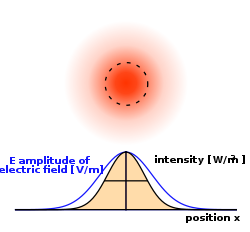
Instantaneous intensity of a Gaussian beam.

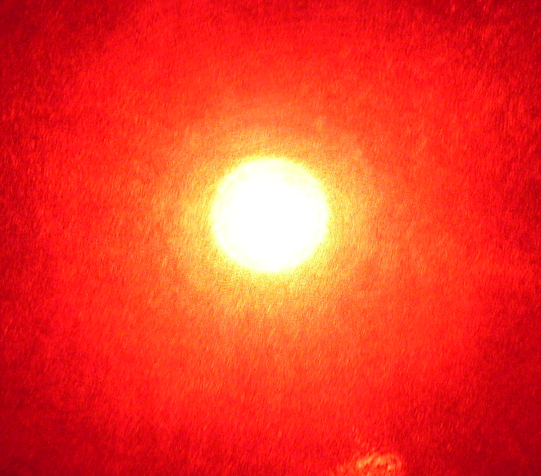
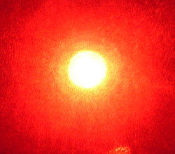Light from a 630 nm laser pointer.

The mathematical function that describes the Gaussian beam is a solution to the paraxial form of the Helmholtz equation. The solution, in the form of a Gaussian function, represents the complex amplitude of the beam's electric field. The electric field and magnetic field together propagate as an electromagnetic wave. A description of just one of the two fields is sufficient to describe the properties of the beam.

Mathematical form

For a Gaussian beam, the complex electric field amplitude is given by

$E(r,z) = E_0 \frac{w_0}{w(z)} \exp \left( \frac{-r^2}{w^2(z)}\right) \exp \left( -ikz -ik \frac{r^2}{2R(z)} +i \zeta(z) \right)\ ,$

where

r is the radial distance from the center axis of the beam,

z is the axial distance from the beam's narrowest point (the "waist"),

i is the imaginary unit (for which i² = − 1),

$k = { 2 \pi \over \lambda }$ is the wave number (in radians per meter),

E₀ = | E(0,0) | ,

w(z) is the radius at which the field amplitude and intensity drop to 1/e and 1/e² of their axial values, respectively,

w₀ = w(0) is the waist size,

R(z) is the radius of curvature of the beam's wavefronts, and

ζ(z) is the Gouy phase shift, an extra contribution to the phase that is seen in Gaussian beams.

The corresponding time-averaged intensity (or irradiance) distribution is

$I(r,z) = { |E(r,z)|^2 \over 2 \eta } = I_0 \left( \frac{w_0}{w(z)} \right)^2 \exp \left( \frac{-2r^2}{w^2(z)} \right)\ ,$

where I₀ = I(0,0) is the intensity at the center of the beam at its waist. The constant $\eta \,$ is the characteristic impedance of the medium in which the beam is propagating. For free space, $\eta = \eta_0 = \sqrt{\frac{\mu_0}{\varepsilon_0}} = 1/(\varepsilon_0 c) \approx 376.7 \ \mathrm{\Omega}$.

Beam parameters

The geometry and behavior of a Gaussian beam are governed by a set of beam parameters, which are defined in the following sections.

Beam width or spot size

See also: Beam diameter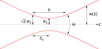

Gaussian beam width w(z) as a function of the axial distance z. w₀: beam waist; b: depth of focus; z_R: Rayleigh range; Θ: total angular spread

For a Gaussian beam propagating in free space, the spot size w(z) will be at a minimum value w₀ at one place along the beam axis, known as the beam waist. For a beam of wavelength λ at a distance z along the beam from the beam waist, the variation of the spot size is given by

$w(z) = w_0 \, \sqrt{ 1+ {\left( \frac{z}{z_\mathrm{R}} \right)}^2 } \ .$

where the origin of the z-axis is defined, without loss of generality, to coincide with the beam waist, and where

$z_\mathrm{R} = \frac{\pi w_0^2}{\lambda}$

is called the Rayleigh range.

Rayleigh range and confocal parameter

At a distance from the waist equal to the Rayleigh range z_R, the width w of the beam is

$w(\pm z_\mathrm{R}) = w_0 \sqrt{2}. \,$

The distance between these two points is called the confocal parameter or depth of focus of the beam:

$b = 2 z_\mathrm{R} = \frac{2 \pi w_0^2}{\lambda}\ .$

Radius of curvature

R(z) is the radius of curvature of the wavefronts comprising the beam. Its value as a function of position is

$R(z) = z \left[{ 1+ {\left( \frac{z_\mathrm{R}}{z} \right)}^2 } \right] \ .$

Beam divergence

The parameter w(z) approaches a straight line for $z \gg z_\mathrm{R}$. The angle between this straight line and the central axis of the beam is called the divergence of the beam. It is given by

$\theta \simeq \frac{\lambda}{\pi w_0} \qquad (\theta \mathrm{\ in\ radians}).$

The total angular spread of the beam far from the waist is then given by

$\Theta = 2 \theta\ .$

Because of this property, a Gaussian laser beam that is focused to a small spot spreads out rapidly as it propagates away from that spot. To keep a laser beam very well collimated, it must have a large diameter. This relationship between beam width and divergence is due to diffraction. Non-Gaussian beams also exhibit this effect, but a Gaussian beam is a special case where the product of width and divergence is the smallest possible.

Since the gaussian beam model uses the paraxial approximation, it fails when wavefronts are tilted by more than about 30° from the direction of propagation.^[1] From the above expression for divergence, this means the Gaussian beam model is valid only for beams with waists larger than about 2λ/π.

Laser beam quality is quantified by the beam parameter product (BPP). For a Gaussian beam, the BPP is the product of the beam's divergence and waist size w₀. The BPP of a real beam is obtained by measuring the beam's minimum diameter and far-field divergence, and taking their product. The ratio of the BPP of the real beam to that of an ideal Gaussian beam at the same wavelength is known as M² ("M squared"). The M² for a Gaussian beam is one. All real laser beams have M² values greater than one, although very high quality beams can have values very close to one.

Gouy phase

The longitudinal phase delay or Gouy phase of the beam is

$\zeta(z) = \arctan \left( \frac{z}{z_\mathrm{R}} \right) \ .$

This phase shifts by π as the beam passes through the focus, in addition to the normal change in phase as the beam propagates.

Complex beam parameter

Main article: Complex beam parameter

The complex beam parameter is

$q(z) = z + q_0 = z + iz_\mathrm{R} \ .$

It is often convenient to calculate this quantity in terms of its reciprocal:

${ 1 \over q(z) } = { 1 \over z + iz_\mathrm{R} } = { z \over z^2 + z_\mathrm{R}^2 } - i { z_\mathrm{R} \over z^2 + z_\mathrm{R}^2 } = {1 \over R(z) } - i { \lambda \over \pi w^2(z) }.$

The complex beam parameter plays a key role in the analysis of gaussian beam propagation, and especially in the analysis of optical resonator cavities using ray transfer matrices.

In terms of the complex beam parameter q, a Gaussian field with one transverse dimension is proportional to

${u}(x,z) = \frac{1}{\sqrt{{q}_x(z)}} \exp\left(-i k \frac{x^2}{2 {q}_x(z)}\right).$

In two dimensions one can write the potentially elliptical or astigmatic beam as the product

${u}(x,y,z) = {u}(x,z)\, {u}(y,z),$

which for the common case of circular symmetry where q_x = q_y = q and x² + y² = r² yields^[2]

${u}(r,z) = \frac{1}{{q}(z)}\exp\left( -i k\frac{r^2}{2 {q}(z)}\right).$

Power and intensity

Power through an aperture

The power P passing through a circle of radius r in the transverse plane at position z is

$P(r,z) = P_0 \left[ 1 - e^{-2r^2 / w^2(z)} \right]\ ,$

where

$P_0 = { 1 \over 2 } \pi I_0 w_0^2$

is the total power transmitted by the beam.

For a circle of radius $r = w(z) \,$, the fraction of power transmitted through the circle is

${ P(z) \over P_0 } = 1 - e^{-2} \approx 0.865\ .$

Similarly, about 95 percent of the beam's power will flow through a circle of radius $r = 1.224\cdot w(z) \,$.

Peak and average intensity

The peak intensity at an axial distance z from the beam waist is calculated using L'Hôpital's rule as the limit of the enclosed power within a circle of radius r, divided by the area of the circle πr²:

$I(0,z) =\lim_{r\to 0} \frac {P_0 \left[ 1 - e^{-2r^2 / w^2(z)} \right]} {\pi r^2} = \frac{P_0}{\pi} \lim_{r\to 0} \frac { \left[ -(-2)(2r) e^{-2r^2 / w^2(z)} \right]} {w^2(z)(2r)} = {2P_0 \over \pi w^2(z)}.$

The peak intensity is thus exactly twice the average intensity, obtained by dividing the total power by the area within the radius w(z).

Higher-order modes

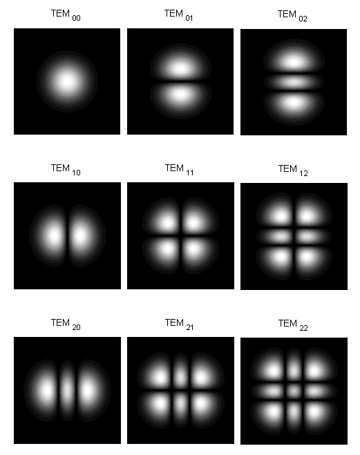
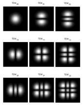The first nine Hermite-Gaussian modes

See also: Transverse mode

Gaussian beams are just one possible solution to the paraxial wave equation. Various other sets of orthogonal solutions are used for modelling laser beams. In the general case, if a complete basis set of solutions is chosen, any real laser beam can be described as a superposition of solutions from this set. The design of the laser determines which basis set of solutions is most useful. In some cases the output of a laser may closely approximate a single higher-order mode. Hermite-Gaussian modes are particularly common, since many laser systems have Cartesian reflection symmetry in the plane perpendicular to the beam's propagation direction.

Hermite-Gaussian modes

Hermite-Gaussian modes are a convenient description for the output of lasers whose cavity design is not radially symmetric, but rather has a distinction between horizontal and vertical. In terms of the previously defined complex q parameter, the intensity distribution in the x-plane is proportional to

${u}_n(x,z) = \left(\frac{2}{\pi}\right)^{1/4} \left(\frac{1}{2^n n! w_0}\right)^{1/2} \left( \frac{{q}_0}{{q}(z)}\right)^{1/2} \left[\frac{{q}_0}{{q}_0^\ast} \frac{{q}^\ast(z)}{{q}(z)}\right]^{n/2} H_n\left(\frac{\sqrt{2}x}{w(z)}\right) \exp\left[-i \frac{k x^2}{2 {q}(z)}\right]$

where the function H_n(x) is the Hermite polynomial of order n (physicists' form, i.e. $H_1(x)=2x\,$), and the asterisk indicates complex conjugation. For the case n = 0 the equation yields a Gaussian transverse distribution.

For two-dimensional rectangular coordinates one constructs a function u_m,n(x,y,z) = u_m(x,z)u_n(y,z), where u_n(y,z) has the same form as u_m(x,z). Mathematically this property is due to the separation of variables applied to the paraxial Helmholtz equation for Cartesian coordinates.^[3]

Hermite-Gaussian modes are typically designated "TEM_m,n", where m and n are the polynomial indices in the x and y directions. A Gaussian beam is thus TEM_0,0.

Laguerre-Gaussian modes

If the problem is cylindrically symmetric, the natural solution of the paraxial wave equation are Laguerre-Gaussian modes. They are written in cylindrical coordinates using Laguerre polynomials

${u}(r,\phi,z)=\frac{C^{LG}_{lp}}{w(z)}\left(\frac{r \sqrt{2}}{w(z)}\right)^{|l|}\exp\left(-\frac{r^2}{w^2(z)}\right)L_p^{|l|} \left(\frac{2r^2}{w^2(z)}\right) \exp\left( i k \frac{r^2}{2 R(z)}\right)\exp(i l \phi)\exp\left[-i(2p+|l|+1)\zeta(z)\right],$

where $L_p^l$ are the generalized Laguerre polynomials, the radial index $p\ge 0$ and the azimuthal index is l. $C^{LG}_{lp}$ is an appropriate normalization constant; w(z), R(z) and ζ(z) are beam parameters defined above.

Ince-Gaussian modes

In elliptic coordinates, one can write the higher-order modes using Ince polynomials. The even and odd Ince-Gaussian modes are given by ^[4]

$u_\varepsilon \left( \xi ,\eta ,z\right) = \frac{w_{0}}{w\left( z\right) }\mathrm{C}_{p}^{m}\left( i\xi ,\varepsilon \right) \mathrm{C} _{p}^{m}\left( \eta ,\varepsilon \right) \exp \left[ -ik\frac{r^{2}}{ 2q\left( z\right) }-\left( p+1\right) \psi _{GS}\left( z\right) \right] ,$

where ξ and η are the radial and angular elliptic coordinates defined by

$x = \sqrt{\varepsilon /2}w\left( z\right) \cosh \xi \cos \eta ,$

$y = \sqrt{\varepsilon /2}w\left( z\right) \sinh \xi \sin \eta.$

${C}_{p}^{m}\left( \eta ,\epsilon \right)$ are the even Ince polynomials of order p and degree m, ε is the ellipticity parameter, and $\psi _{GS}\left( z\right) =\arctan \left( z/z_\mathrm{R}\right)$ is the Gouy phase. The Hermite-Gaussian and Laguerre-Gaussian modes are a special case of the Ince-Gaussian modes for $\varepsilon=\infty$ and ε = 0 respectively.

Hypergeometric-Gaussian modes

There is another important class of paraxial wave modes in the polar coordinates in which its complex amplitude is proportional to confluent Hypergeometric function. These modes have a singular phase profile and are eigenfunctions of the photon orbital angular momentum. The intensity profile is characterized by a single brilliant ring with the singularity at its center, where the field amplitude vanishes ^[5]

$u_{pm}(\rho,\theta;\zeta)= \sqrt{\frac{2^{p+|m|+1}}{\pi\Gamma(p+|m|+1)}} \frac{\Gamma(1+|m|+\frac{p}{2})}{\Gamma(|m|+1)} \,\,i^{|m|+1}\zeta^{\frac{p}{2}}(\zeta+i)^{-(1+|m|+\frac{p}{2})}\rho^{|m|}e^{-\frac{i\rho^2}{(\zeta+i)}}e^{im\phi}{}_{1}F_{1}\left(-\frac{p}{2}, |m|+1;\frac{r^2}{\zeta(\zeta+i)}\right),$

where m is integer, $p\ge-|m|$ is real valued, Γ(x) is the gamma function and ₁F₁(a,b;x) is a confluent hypergeometric function. Some subfamilies of the Hypergeometric-Gaussian (HyGG) modes can be listed as the modified Bessel Gaussian modes, the modified exponential Gaussian modes, and the modified Laguerre–Gaussian modes. However, the HyGG is overcomplete and it is not orthogonal set of modes. In spite of its complicated field profile, HyGG modes have a very simple profile at the pupil plane (see optical vortex):

$u(\rho,\phi,0) \propto \rho^{p+|m|}e^{-\rho^2+im\phi},$

where it explains that out coming wave from pitch-fork hologram is a sub family of HyGG modes. The HyGG profile while beam propagates along ζ has a dramatic change and it is not stable mode below the Rayleigh range.

See also

• Gaussian function
• Electromagnetic wave equation
• Hermite polynomials
• Laguerre polynomials
• Bessel beam
• Tophat beam
• Laser beam profiler

Notes

1. ^ Siegman (1986) p. 630.
2. ^ See Siegman (1986) p. 639. Eq. 29
3. ^ Siegman (1986), p645, eq. 54
4. ^ Bandres and Gutierrez-Vega (2004)
5. ^ Karimi et. al (2007)

References

• Saleh, Bahaa E. A. and Teich, Malvin Carl (1991). Fundamentals of Photonics. New York: John Wiley & Sons. ISBN 0-471-83965-5.  Chapter 3, "Beam Optics," pp. 80–107.

• Mandel, Leonard and Wolf, Emil (1995). Optical Coherence and Quantum Optics. Cambridge: Cambridge University Press. ISBN 0-521-41711-2.  Chapter 5, "Optical Beams," pp. 267.

• Siegman, Anthony E. (1986). Lasers. University Science Books. ISBN 0-935702-11-3.  Chapter 16.

• Yariv, Amnon (1989). Quantum Electronics (3rd ed.). Wiley. ISBN 0-471-60997-8. 

• F. Pampaloni and J. Enderlein (2004). "Gaussian, Hermite-Gaussian, and Laguerre-Gaussian beams: A primer". arXiv:physics/0410021 [physics.optics]. 

• Miguel A. Bandres and Julio C. Gutierrez-Vega (2004). "Ince Gaussian beams". Opt. Lett. (OSA) 29 (2): 144–146. Bibcode 2004OptL...29..144B. doi:10.1364/OL.29.000144. PMID 14743992. http://www.opticsinfobase.org/abstract.cfm?URI=ol-29-2-144. 
• E. Karimi, G. Zito, B. Piccirillo, L. Marrucci, and E. Santamato (2007). "Hypergeometric-Gaussian beams". Opt. Lett. (OSA) 32 (21): 3053–3055. Bibcode 2007OptL...32.3053K. doi:10.1364/OL.32.003053. PMID 17975594. http://www.opticsinfobase.org/abstract.cfm?URI=ol-32-21-3053. 
• Gaussian Beam Propagation - CVI Melles Griot Technical Guide
• Gaussian Beam Optics Tutorial, Newport