Motion graphs and derivatives

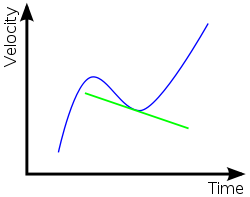The green line shows the slope of the velocity-time graph at the particular point where the two lines touch. Its slope is the acceleration at that point.

In mechanics, the derivative of the position vs. time graph of an object is equal to the velocity of the object. In the International System of Units, the position of the moving object is measured in meters relative to the origin, while the time is measured in seconds. Placing position on the y-axis and time on the x-axis, the slope of the curve is given by:

$v = \frac{\Delta y}{\Delta x} = \frac{\Delta s}{\Delta t}.$

Here s is the position of the object, and t is the time. Therefore, the slope of the curve gives the change in position (in metres) divided by the change in time (in seconds), which is the definition of the average velocity (in meters per second $(\begin{matrix} \frac{m}{s} \end{matrix})$) for that interval of time on the graph. If this interval is made to be infinitesimally small, such that Δs becomes ds and Δt becomes dt, the result is the instantaneous velocity at time t, or the derivative of the position with respect to time.

A similar fact also holds true for the velocity vs. time graph. The slope of a velocity vs. time graph is acceleration, this time, placing velocity on the y-axis and time on the x-axis. Again the slope of a line is change in y over change in x:

$a = \frac{\Delta y}{\Delta x} = \frac{\Delta v}{\Delta t}.$

Where v is the velocity, measured in $\begin{matrix} \frac{m}{s} \end{matrix}$, and t is the time measured in seconds. This slope therefore defines the average acceleration over the interval, and reducing the interval infinitesimally gives $\begin{matrix} \frac{dv}{dt} \end{matrix}$, the instantaneous acceleration at time t, or the derivative of the velocity with respect to time (or the second derivative of the position with respect to time). The units of this slope or derivative are in meters per second per second ($\begin{matrix} \frac{m}{s^2} \end{matrix}$, usually termed "meters per second-squared"), and so, therefore, is the acceleration.

Since the velocity of the object is the derivative of the position graph, the area under the line in the velocity vs. time graph is the displacement of the object. (Velocity is on the y-axis and time on the x-axis. Multiplying the velocity by the time, the seconds cancel out and only meters remain. $\begin{matrix} \frac{m}{s} \end{matrix}s = m$.)

The same multiplication rule holds true for acceleration vs. time graphs. When $(\begin{matrix} \frac{m}{s^2} \end{matrix})$ is multiplied by time (s), velocity is obtained. ($\begin{matrix} \frac{m}{s^2} \end{matrix}s = \begin{matrix} \frac{m}{s} \end{matrix}$).

Variable rates of change

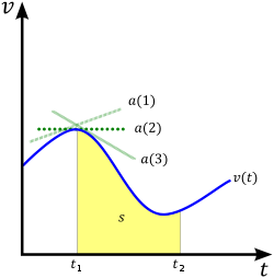In this example, the yellow area represents the displacement of the object as it moves. (The distance can be measured by taking the absolute value of the function.) The three green lines represent the values for acceleration at different points along the curve.

The expressions given above apply only when the rate of change is constant or when only the average (mean) rate of change is required. If the velocity or positions change non-linearly over time, such as in the example shown in the figure, then differentiation provides the correct solution. Differentiation reduces the time-spans used above to be extremely small and gives a velocity or acceleration at each point on the graph rather than between a start and end point. The derivative forms of the above equations are

$v = \frac{ds}{dt},$

$a = \frac{dv}{dt}.$

Since acceleration differentiates the expression involving position, it can be rewritten as a second derivative with respect to position:

$a = \frac{d^2 s}{dt^2}.$

Since, for the purposes of mechanics such as this, integration is the opposite of differentiation, it is also possible to express position as a function of velocity and velocity as a function of acceleration. The process of determining the area under the curve, as described above, can give the displacement and change in velocity over particular time intervals by using definite integrals:

$s(t_2)-s(t_1) = \int_{t_1}^{t_2}{v}\, dt,$

$v(t_2)-v(t_1) = \int_{t_1}^{t_2}{a}\, dt.$

See also

• Displacement (vector)
• Velocity
• Acceleration
• Kinematics

References

• Wolfson, Richard; Jay M. Pasachoff (1999). Physics for Scientists and Engineers (3rd ed. ed.). Reading, Massachusetts: Addison-Wesley. pp. 23–38. ISBN 0-321-03571-2.