Difference-map algorithm

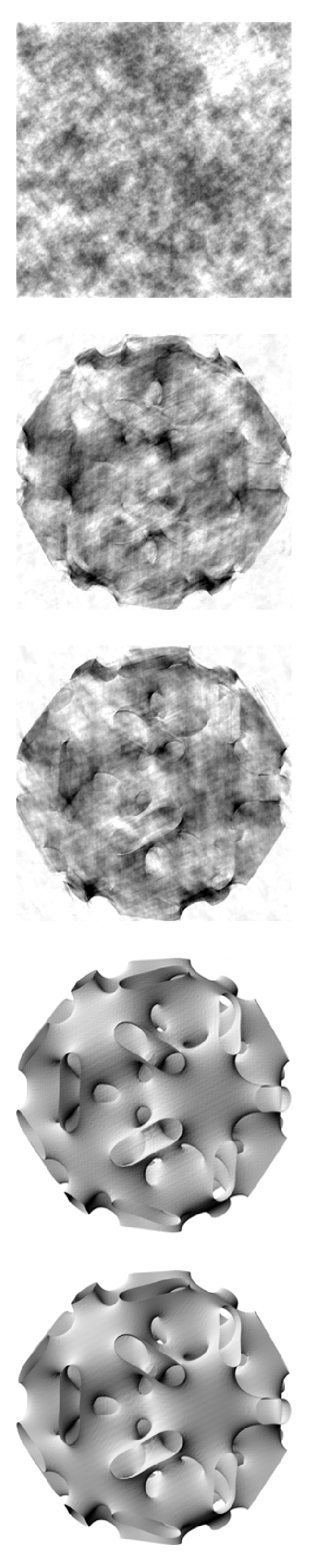
Iterations 0, 100, 200, 300 and 400 in the difference-map reconstruction of a grayscale image from its Fourier transform modulus

The difference-map algorithm is a search algorithm for general constraint satisfaction problems. It is a meta-algorithm in the sense that it is built from more basic algorithms that perform projections onto constraint sets. From a mathematical perspective, the difference-map algorithm is a dynamical system based on a mapping of Euclidean space. Solutions are encoded as fixed points of the mapping.

Although originally conceived as a general method for solving the phase problem, the difference-map algorithm has been used for the boolean satisfiability problem, protein structure prediction, Ramsey numbers, diophantine equations, and Sudoku^[1], as well as sphere- and disk-packing problems^[2]. Since these applications include NP-complete problems, the scope of the difference map is that of an incomplete algorithm. Whereas incomplete algorithms can efficiently verify solutions (once a candidate is found), they cannot prove that a solution does not exist.

The difference-map algorithm is a generalization of two iterative methods: Fienup's Hybrid input output (HIO) algorithm for phase retrieval ^[3] and the Douglas-Rachford algorithm^[4] for convex optimization. Iterative methods, in general, have a long history in phase retrieval and convex optimization. The use of this style of algorithm for hard, non-convex problems is a more recent development.

Algorithm

The problem to be solved must first be formulated as a set intersection problem in Euclidean space: find an x in the intersection of sets A and B. Another prerequisite is an implementation of the projections P_A and P_B that, given an arbitrary input point x, return a point in the constraint set A or B that is nearest to x. One iteration of the algorithm is given by the mapping:

x → D(x) = x + β [ P_A( f_B(x)) - P_B( f_A(x)) ] ,

f_A(x) = P_A(x) - (P_A(x)-x)/β ,

f_B(x) = P_B(x) + (P_B(x)-x)/β .

The real parameter β can have either sign; optimal values depend on the application and are determined through experimentation. As a first guess, the choice β = 1 (or β = -1) is recommended because it reduces the number of projection computations per iteration:

D(x) = x + P_A(2 P_B(x) - x) - P_B(x) .

The progress of the algorithm is monitored by inspecting the norm of the difference of the two projections:

Δ = | P_A( f_B(x)) - P_B( f_A(x)) | .

When this vanishes, at fixed points of the map, a point common to both constraint sets has been found and the algorithm is terminated. The set of fixed points in a particular application will normally have a large dimension, even when the solution set is a single point.

Example: logical satisfiability

Incomplete algorithms, such as stochastic local search, are widely used for finding satisfying truth assignments to boolean formulas. As an example of solving an instance of 2-SAT with the difference-map algorithm, consider the following formula (~ indicates NOT):

(q₁ or q₂) and (~q₁ or q₃) and (~q₂ or ~q₃) and (q₁ or ~q₂)

To each of the eight literals in this formula we assign one real variable in an eight dimensional Euclidean space. The structure of the 2-SAT formula can be recovered when these variables are arranged in a table:

x11	x12
(x21)		x22
	(x31)	(x32)
x41	(x42)

Rows are the clauses in the 2-SAT formula and literals corresponding to the same boolean variable are arranged in columns, with negation indicated by parentheses. For example, the real variables x₁₁, x₂₁ and x₄₁ correspond to the same boolean variable (q₁) or its negation, and are called replicas. It is convenient to associate the values 1 and -1 with TRUE and FALSE rather than the traditional 1 and 0. With this convention, the compatibility between the replicas takes the form of the following linear equations:

x₁₁ = -x₂₁ = x₄₁

x₁₂ = -x₃₁ = -x₄₂

x₂₂ = -x₃₂

The linear subspace where these equations are satisfied is one of the constraint spaces, say A, used by the difference map. To project to this constraint we replace each replica by the signed replica average, or its negative:

a₁ = (x₁₁ - x₂₁ + x₄₁) / 3

x₁₁ → a₁   x₂₁ → -a₁   x₄₁ → a₁

The second difference-map constraint applies to the rows of the table, the clauses. In a satisfying assignment, the two variables in each row must be assigned the values (1, 1), (1, -1), or (-1, 1). The corresponding constraint set, B, is thus a set of 3⁴ = 81 points. In projecting to this constraint the following operation is applied to each row. First, the two real values are rounded to 1 or -1; then, if the outcome is (-1, -1), the larger of the two original values is replaced by 1. Examples:

(-.2, 1.2) → (-1, 1)

(-.2, -.8) → (1, -1)

It is a straightforward exercise to check that both of the projection operations described minimize the Euclidean distance between input and output values. Moreover, if the algorithm succeeds in finding a point x that lies in both constraint sets, then we know that (i) the clauses associated with x are all TRUE, and (ii) the assignments to the replicas are consistent with a truth assignment to the original boolean variables.

To run the algorithm one first generates an initial point x₀, say

-0.5	-0.8
(-0.4)		-0.6
	(0.3)	(-0.8)
0.5	(0.1)

Using β = 1, the next step is to compute P_B(x₀) :

1	-1
(1)		-1
	(1)	(-1)
1	(1)

This is followed by 2P_B(x₀) - x₀,

2.5	-1.2
(2.4)		-1.4
	(1.7)	(-1.2)
1.5	(1.9)

and then projected onto the other constraint, P_A(2P_B(x₀) - x₀) :

0.53333	-1.6
(-0.53333)		-0.1
	(1.6)	(0.1)
0.53333	(1.6)

Incrementing x₀ by the difference of the two projections gives the first iteration of the difference map, D(x₀) = x₁ :

-0.96666	-1.4
(-1.93333)		0.3
	(0.9)	(0.3)
0.03333	(0.7)

Here is the second iteration, D(x₁) = x₂ :

-0.3	-1.4
(-2.6)		-0.7
	(0.9)	(-0.7)
0.7	(0.7)

This is a fixed point: D(x₂) = x₂. The iterate is unchanged because the two projections agree. From P_B(x₂) ,

1	-1
(-1)		1
	(1)	(-1)
1	(1)

we can read off the satisfying truth assignment: q₁ = TRUE, q₂ = FALSE, q₃ = TRUE.

Chaotic dynamics

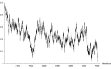Time series of the norm of the difference-map increment Δ in the course of solving a random 3-SAT instance with 1000 variables and 4200 clauses.

In the simple 2-SAT example above, the norm of the difference-map increment Δ decreased monotonically to zero in three iterations. This contrasts the behavior of Δ when the difference map is given a hard instance of 3-SAT, where it fluctuates strongly prior to the discovery of the fixed point. As a dynamical system the difference map is believed to be chaotic, and that the space being searched is a strange attractor.

Phase retrieval

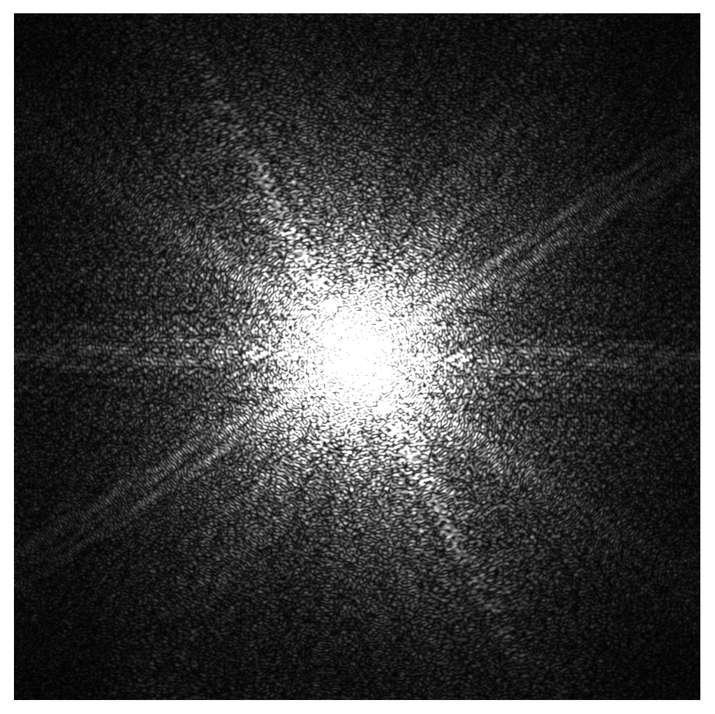
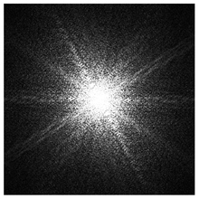Fourier transform modulus (diffraction pattern) of the grayscale image shown being reconstructed at the top of the page.

In phase retrieval a signal or image is reconstructed from the modulus (absolute value, magnitude) of its discrete Fourier transform. For example, the source of the modulus data may be the Fraunhofer diffraction pattern formed when an object is illuminated with coherent light.

The projection to the Fourier modulus constraint, say P_A, is accomplished by first computing the discrete Fourier transform of the signal or image, rescaling the moduli to agree with the data, and then inverse transforming the result. This is a projection, in the sense that the Euclidean distance to the constraint is minimized, because (i) the discrete Fourier transform, as a unitary transformation, preserves distance, and (ii) rescaling the modulus (without modifying the phase) is the smallest change that realizes the modulus constraint.

To recover the unknown phases of the Fourier transform the difference map relies on the projection to another constraint, P_B. This may take several forms, as the object being reconstructed may be known to be positive, have a bounded support, etc. In the reconstruction of the surface image, for example, the effect of the projection P_B was to nullify all values outside a rectangular support, and also to nullify all negative values within the support.

Notes

1. ^ V. Elser, I. Rankenburg, and P. Thibault, "Searching with iterated maps". Proceedings of the National Academy of Sciences USA. (2007). 104:418-423. http://www.pnas.org/cgi/content/short/104/2/418
2. ^ S. Gravel, V. Elser, "Divide and concur: A general approach to constraint satisfaction". Physical Review E. (2008). 78:036706. http://link.aps.org/doi/10.1103/PhysRevE.78.036706
3. ^ J.R. Fienup, "Phase retrieval algorithms: a comparison". Applied Optics. (1982). 21:2758-2769.
4. ^ H.H. Bauschke, P.L. Combettes, and D.R. Luke, "Phase retrieval, error reduction algorithm, and Fienup variants: a view from convex optimization". Journal of the Optical Society of America A. (2002). 19:1334-1345.