Discretization

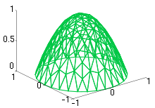
A solution to a discretized partial differential equation, obtained with the finite element method.

In mathematics, discretization concerns the process of transferring continuous models and equations into discrete counterparts. This process is usually carried out as a first step toward making them suitable for numerical evaluation and implementation on digital computers. In order to be processed on a digital computer another process named quantization is essential.

• Euler discretization
• Zero-order hold

Discretization is also related to discrete mathematics, and is an important component of granular computing. In this context, discretization may also refer to modification of variable of category granularity, as when multiple discrete variables are aggregated or multiple discrete categories fused.

Discretization of linear state space models

Discretization is also concerned with the transformation of continuous differential equations into discrete difference equations, suitable for numerical computing.

The following continuous-time state space model

$\dot{\mathbf{x}}(t) = \mathbf A \mathbf{x}(t) + \mathbf B \mathbf{u}(t) + \mathbf{w}(t)$

$\mathbf{y}(t) = \mathbf C \mathbf{x}(t) + \mathbf D \mathbf{u}(t) + \mathbf{v}(t)$

where v and w are continuous zero-mean white noise sources with covariances

$\mathbf{w}(t) \sim N(0,\mathbf Q)$

$\mathbf{v}(t) \sim N(0,\mathbf R)$

can be discretized, assuming zero-order hold for the input u and continuous integration for the noise v, to

$\mathbf{x}[k+1] = \mathbf A_d \mathbf{x}[k] + \mathbf B_d \mathbf{u}[k] + \mathbf{w}[k]$

$\mathbf{y}[k] = \mathbf C_d \mathbf{x}[k] + \mathbf D_d \mathbf{u}[k] + \mathbf{v}[k]$

with covariances

$\mathbf{w}[k] \sim N(0,\mathbf Q_d)$

$\mathbf{v}[k] \sim N(0,\mathbf R_d)$

where

$\mathbf A_d = e^{\mathbf A T} = \mathcal{L}^{-1}\{(s\mathbf I - \mathbf A)^{-1}\}_{t=T}$

$\mathbf B_d = \left( \int_{\tau=0}^{T}e^{\mathbf A \tau}d\tau \right) \mathbf B = \mathbf A^{-1}(\mathbf A_d - I)\mathbf B$, if $\mathbf A$ is nonsingular

$\mathbf C_d = \mathbf C$

$\mathbf D_d = \mathbf D$

$\mathbf Q_d = \int_{\tau=0}^{T} e^{\mathbf A \tau} \mathbf Q e^{\mathbf A^T \tau} d\tau$

$\mathbf R_d = \mathbf R$

and T is the sample time.

A clever trick to compute Ad and Bd in one step is by utilizing the following property, p. 215 ^[1]:

$\mathbf e^{\mathbf \begin{bmatrix} \mathbf{A} & \mathbf{B} \\ \mathbf{0} & \mathbf{0} \end{bmatrix} T} = \begin{bmatrix} \mathbf{M_{11}} & \mathbf{M_{12}} \\ \mathbf{0} & \mathbf{I} \end{bmatrix}$

and then having

$\mathbf A_d = M_{11}$

$\mathbf B_d = M_{12}$

Discretization of process noise

Numerical evaluation of $\mathbf{Q}_d$ is a bit trickier due to the matrix exponential integral. It can, however, be computed by first constructing a matrix, and computing the exponential of it (Van Loan, 1978):

$\mathbf{F} = \begin{bmatrix} -\mathbf{A} & \mathbf{Q} \\ \mathbf{0} & \mathbf{A}^T \end{bmatrix} T$

$\mathbf{G} = e^\mathbf{F} = \begin{bmatrix} \dots & \mathbf{A}_d^{-1}\mathbf{Q}_d \\ \mathbf{0} & \mathbf{A}_d^T \end{bmatrix}.$

The discretized process noise is then evaluated by multiplying the transpose of the lower-right partition of G with the upper-right partition of G:

$\mathbf{Q}_d = (\mathbf{A}_d^T)^T (\mathbf{A}_d^{-1}\mathbf{Q}_d).$

Derivation

Starting with the continuous model

$\mathbf{\dot{x}}(t) = \mathbf A\mathbf x(t) + \mathbf B \mathbf u(t)$

we know that the matrix exponential is

$\frac{d}{dt}e^{\mathbf At} = \mathbf A e^{\mathbf At} = e^{\mathbf At} \mathbf A$

and by premultiplying the model we get

$e^{-\mathbf At} \mathbf{\dot{x}}(t) = e^{-\mathbf At} \mathbf A\mathbf x(t) + e^{-\mathbf At} \mathbf B\mathbf u(t)$

which we recognize as

$\frac{d}{dt}(e^{-\mathbf At}\mathbf x(t)) = e^{-\mathbf At} \mathbf B\mathbf u(t)$

and by integrating..

$e^{-\mathbf At}\mathbf x(t) - e^0\mathbf x(0) = \int_0^t e^{-\mathbf A\tau}\mathbf B\mathbf u(\tau) d\tau$

$\mathbf x(t) = e^{\mathbf At}\mathbf x(0) + \int_0^t e^{\mathbf A(t-\tau)} \mathbf B\mathbf u(\tau) d \tau$

which is an analytical solution to the continuous model.

Now we want to discretise the above expression. We assume that u is constant during each timestep.

$\mathbf x[k] \ \stackrel{\mathrm{def}}{=}\ \mathbf x(kT)$

$\mathbf x[k] = e^{\mathbf AkT}\mathbf x(0) + \int_0^{kT} e^{\mathbf A(kT-\tau)} \mathbf B\mathbf u(\tau) d \tau$

$\mathbf x[k+1] = e^{\mathbf A(k+1)T}\mathbf x(0) + \int_0^{(k+1)T} e^{\mathbf A((k+1)T-\tau)} \mathbf B\mathbf u(\tau) d \tau$

$\mathbf x[k+1] = e^{\mathbf AT} \left[ e^{\mathbf AkT}\mathbf x(0) + \int_0^{kT} e^{\mathbf A(kT-\tau)} \mathbf B\mathbf u(\tau) d \tau \right]+ \int_{kT}^{(k+1)T} e^{\mathbf A(kT+T-\tau)} \mathbf B\mathbf u(\tau) d \tau$

We recognize the bracketed expression as $\mathbf x[k]$, and the second term can be simplified by substituting v = kT + T − τ. We also assume that $\mathbf u$ is constant during the integral, which in turn yields

$\mathbf x[k+1] = e^{\mathbf AT}\mathbf x[k] + \left( \int_0^T e^{\mathbf Av} dv \right) \mathbf B\mathbf u[k]=e^{\mathbf AT}\mathbf x[k] + A^{-1}\left(e^{\mathbf AT}-I \right) \mathbf B\mathbf u[k]$

which is an exact solution to the discretization problem.

Approximations

Exact discretization may sometimes be intractable due to the heavy matrix exponential and integral operations involved. It is much easier to calculate an approximate discrete model, based on that for small timesteps $e^{\mathbf AT} \approx \mathbf I + \mathbf A T$. The approximate solution then becomes:

$\mathbf x[k+1] \approx (\mathbf I + \mathbf AT) \mathbf x[k] + (\mathbf I T + \frac{1}{2} \mathbf A T^2 ) \mathbf B \mathbf u[k]$

which can further be approximated if $\frac{1}{2} \mathbf A T^2$ is small; yielding

$\mathbf x[k+1] \approx (\mathbf I + \mathbf AT) \mathbf x[k] + T\mathbf B \mathbf u[k]$

Other possible approximations are $e^{\mathbf AT} \approx \left( \mathbf I - \mathbf A T \right)^{-1}$ and $e^{\mathbf AT} \approx \left( \mathbf I +\frac{1}{2} \mathbf A T \right) \left( \mathbf I - \frac{1}{2} \mathbf A T \right)^{-1}$. Each of them have different stability properties. The last one is known as the bilinear transform, or Tustin transform, and preserves the (in)stability of the continuous-time system.

Discretization of continuous features

Main article: Discretization of continuous features

In statistics and machine learning, discretization refers to the process of converting continuous features or variables to discretized or nominal features. This can be useful when creating probability mass functions.

See also

• Discrete space
• Time scale calculus

References

1. ^ Raymond DeCarlo: Linear Systems: A State Variable Approach with Numerical Implementation, Prentice Hall, NJ, 1989

• Robert Grover Brown & Patrick Y. C. Hwang: Introduction to random signals and applied Kalman filtering, 3rd ed.
• Chi-Tsong Chen: Linear System Theory and Design.
• C. Van Loan: Computing integrals involving the matrix exponential, IEEE Transactions on Automatic Control, vol.23, no.3, pp. 395–404, Jun 1978

External links